- Introduction
- Getting Started
- Python Scripts
- Calibrating SMA Data with CASA
- Imaging SMA Data with CASA
- Getting Help
|
Welcome to the SMA CASA Website. SMA data can be imported directly into CASA (Common Astronomy Software Applications) without any pre-processing in MIR or Miriad. To date, CASA has been tested on single and dual receiver data, and data from the new SWARM (SMA Wideband Astronomical ROACH2 Machine) correlator. It cannot currently handle polarization data.
In the following sections, we convert raw SMA data to CASA measurement set (MS) format, then calibrate and image using SMA-specific CASA software.
|
There are three (3) available sites for running CASA:
- Cambridge
To run CASA on the R&G public machines, e.g., rtdc7, type:
ssh -X rtdc7
casapy42To run CASA on the CF managed machines, e.g., cfa0, type:
ssh -X 131.142.20.100 (if not originating from a CF managed machine)
ssh -Y cfa0
/sma/ALMA/casa-42/casapy
Notes:- It is best to run the latest CASA release, CASA 4.2.0 (above). For other CASA versions, see the R&G CASA website.
- To obtain an account on the CF managed machines, contact: cfhelp@cfa.harvard.edu
- Hawaii
To run CASA on the SMA Hawaii machine hilodr2, type:
ssh -X 128.171.166.107
cd /usr/local/casapy-stable-42.0.26465-011-64b
casapy
Notes:- The stable version (r26945) is not the final version (r28322), i.e., release, of CASA 4.2.0, but it is the only version currently available in Hawaii.
- To obtain an account on the SMA Hawaii machines, contact: smaCASA@cfa.harvard.edu
- Herndon, Virginia
In the near future, users will be able to run their time or cpu intensive jobs using parallelized CASA on the Linux based Beowulf cluster, hydra.
Get the correct version of Python
The CASA data reduction programs (for calibration and imaging) are written in C++ and run via an iPython interface. Python scripts are therefore an integral part of CASA processing.
The scripts written to import SMA data into CASA are compatible with the Anaconda Python distribution (Python 2.7.6), but may work with other distributions, as well. If the scripts
do not work on your machine (e.g., Python 2.6.6 will complain about missing modules), download the Anaconda Python distribution.
An additional resource (for both Linux and Mac) can be found at http://www.Python.org.
You can determine the version of Python running on your machine by typing:
Python -V
Get the necessary Python scripts
Two Python scripts have been written that allow you to import SMA data into CASA.
- sma2casa.py
This script outputs a FITS-IDI file for each sideband of each spectral chunk in the data set. The most recent version of the script can be obtained from the github software depository by typing:
git clone https://github.com/smithsonian/sma2casa.git
Notes:- The script can be run as is on any of the CF managed Linux machines (see above). If running elsewhere, change the script's first line to point to your local Python distribution.
- There are two (2) ways to run the script:
- By default, sma2casa.py will call the module makevis.c, which requires that makevis.so be present in your current working directory. If it is not, or if sma2casa.py does not work properly, you can recompile makevis.c from source code and a Makefile in the github repository.
- Alternatively, the script can be run with the -P option. This option has the advantage of being more portable (no recompiling necessary), but the disadvantage of running more slowly (by ~ a factor of 2).
- The following Python modules must be present:
numpy
To verify that they are installed, type (on successive lines):
astropy
pyfits (now a part of astropy)Python
If you don't have the necessary Python modules, install the Anaconda Python distribution, which has everything needed for running sma2casa.py.
help()
modules
- smaimportFix.py
This script reads the FITS-IDI files output by sma2casa.py and writes them to CASA Measurement Set (MS) format. A single output file is produced.
Notes:-
If you get the error message:
NameError: name 'tflagdata' is not defined,
change "tflagdata" to "flagdata" in the smaimportFix.py script. CASA 4.2.0 stable (r26945) and earlier versions recognize tflagdata; CASA 4.2.0 release (r28322) and later versions do not. -
The following Python modules are part of a standard CASA installation and should be present:
casac
tasks
taskinit
pylab
pyfits
-
If you get the error message:
What the script does
The python script, sma2casa.py,
-
Creates one FITS-IDI file for each sideband of each chunk of a raw SMA data set.
The FITS-IDI files will later be read by a second script, smaimportFix.py, which creates a CASA measurement set (MS). The reason for this two step conversion process is that CASA measurement set format is not a stable target; it can be changed by the CASA software group at any time. FITS-IDI format, on the other hand, is a standard format which is unlikely to change, because doing so would break many existing software packages. See the "Getting Started" section for information about obtaining these scripts. - Uses Tsys information in the SMA dataset to convert SMA visibilities to "pseudo-Jansky" units, which (barring significant problems with the track, e.g., bad pointing) are within ~20% of the correct Jy values. It also uses Tsys, along with integration time, to calculate weights for the visibilities. These calculations are performed before the FITS-IDI files are written.
Script usage
Execute the command:
sma2casa.py [path-to-SMA-data] [options]
Script options
| -c m,n,o [--chunks m,n,o] | Process chunks m, n and o only (comma separated list) | |
| -h [--help] | Print this message and exit | |
| -l [--lower] | Process lower sideband only | |
| -n [--newChunk] | Define a new, synthetic, spectral chunk | |
| -p [--percent] | Percent to trim on band edge (default = 10) | |
| -P [--PythonOnly] | Do not use the C module "makevis" | |
| -r [--receiver] | Specify the receiver for multi-receiver tracks (230, 345, 400 or 650) | |
| -R [--RxFix] | Force the data to be treated as single receiver | |
| -s [--silent] | Run silently unless an error occurs | |
| -t [--trim] | Set the amplitude at chunk edges to 0.0 | |
| -T | -T n=m means use antenna m's Tsys for antenna n | |
| -u [--upper] | Process upper sideband only | |
| -w m,n,o [--without m,n,o] | Do NOT process chunks m, n and o (comma separated list) |
The -T option provides a crude way to handle bad Tsys information. If antenna n has noisy or garbage Tsys values, -T allows antenna m's Tsys to be used instead for that antenna. Dual receiver tracks must use the -r option, and each receiver must be processed separately.
The -n switch allows you to define new, synthetic, spectral "chunks" (spws in CASA terminology) which have different total bandwidths and spectral resolutions. The main purpose for this feature is to allow SWARM chunks to be processed at reduced spectral resolution, especially for continuum projects, in order to reduce the size of the CASA Measurement Sets. Although SWARM chunks are the ones we are most apt to want to resample, the -n option will work with ASIC correlator chunks too. One may produce a synthetic chunk from a chunk which has been excluded with the -w switch; indeed, doing so will probably be the most common use case. The syntax for a synthetic chunk is
-n originalChunk:startChannel:endChannel:nAverageWhere originalChunk is the hardware chunk number (49 or 50 for SWARM), startChannel is the first channel to use in the original, hardware chunk, endChannel is the last channel to use, and nAverage is the number of channels of the original chunk to vector average to produce a single channel in the synthetic chunk. (1 + endChannel - startChannel) must be evenly divisible by nAverage. One can define any number of synthetic chunks. Because the -n option allows for an arbitrary number of synthetic chunks, it needs to be the last parameter on the command line, because it grabs all the remaining text on the line, and attempts to parse it into new syntetic chunk specifications.
Examples for running script
-
Process both sidebands of all chunks in the data set located at /sma/SMAusers/taco/130408_17:20:01/
sma2casa.py /sma/SMAusers/taco/130408_17:20:01/
-
Process data from the upper sideband of the 400 GHz Rx only
sma2casa.py /sma/SMAusers/taco/130408_17:20:01/ -u -r 400
-
Make a FITS-IDI file for the lower sideband of chunks s03, s05 and s20,
if data exists for those chunks (i.e. if the number of channels has not been set to 0 in the restartCorrelator command).
sma2casa.py /sma/SMAusers/taco/130408_17:20:01/ -l -c 3,5,20
-
Make a FITS-IDI file for the lower sideband of chunk s40, and trim the
highest and lowest 10% of the channels by setting their amplitudes to 0.0 (which will ultimately cause them to be flagged bad).
sma2casa.py /sma/SMAusers/taco/130408_17:20:01/ -l -c 40 -t
-
Make a set of FITS-IDI files with the Tsys values for antennas 4 and 5
replaced by the Tsys values for antenna 7.
sma2casa.py /sma/SMAusers/taco/130408_17:20:01/ -T 4=7 -T 5=7
-
Make a set of FITS-IDI files with synthetic SWARM chunks (an no real SWARM chunks)
with the edge 2048 channels chopped off, and points vector averaged in sets of 128.
sma2casa.py /sma/SMAusers/taco/130408_17:20:01/ -w 49,50 -n 49:2048:14335:128 50:2048:14335:128
Script caveats
-
sma2casa.py calls the C language module, makevis, which does the low-level processing of the visibilities data. The object code for this module
is makevis.so and it must be present in your working directory. Since makevis.so is compiled code, it is not as portable as Python code.
If the script does not work properly in this mode, you can do one of the following:
- Recompile makevis.c. The source code and a Makefile are included in the git repository.
- Run the script, sma2casa.py, with the -P option. This will tell the script to use Python code only, but will slow down execution by ~ a factor of 2.
- sma2casa.py maps the entire visibilities data file into RAM. Hence, the script is apt to run very slowly if the computer's available RAM is smaller than the size of the SMA file, sch_read.
What the script does
The python script, smaImportFix.py,
- Makes a list of which FITS-IDI files are in the current directory, so that it knows which chunks should be processed.
- Reads each FITS-IDI file into a separate CASA measurement set (MS).
- Indicates that a data value is bad by setting its amplitude to 0.0. smaImportFix.py runs the flagdata task on the newly created MS in order to explicitly flag those data points bad. Chunk edge channels are also flagged bad in this step, if you passed arguments to sma2casa.py indicating that you wanted to trim edge channels.
- Deletes the FITS-IDI files.
- Fixes the weights. For all chunks except the pseudo-continuum chunk, the CASA importfitsidi file sets the data weights to 1.0. smaImportFix.py fixes this problem and puts the proper weights, proportional to (integration time)/Tsys**2, in the weight table of the MS.
- Generates new scan numbers. In the raw SMA data sets, each timeslice of data stored by the correlator has a unique scan number. CASA MSs usually have scan numbers which change only when the source is changed (helpful in controlling how calibration information is averaged and interpolated). smaImportFix.py therefore generates a new set of scan numbers which increment only when the source changes. This means that there will usually be several integrations which share the same scan number.
- Concatenates individual chunk MSs into a single MS. One such concatenated MS is made for each sideband, MyDataLower and MyDataUpper.
Script caveats
-
There is a strange, intermittent problem with importing Dual-Rx data into CASA. Occasionally, the frequency scale gets set incorrectly. There is a work-around for this issue:
- make an empty directory
- copy the FITS-IDI files into the new directory
- cd to the new directory
- (re)start CASA in the new directory and run the script, smaImportFix.py
- copy the MSs to their permanent location
Remember, this is only required for dual-Rx tracks. - The CASA SYSCAL table has the Tsys values stored in it, but that is probably only useful for plotting the Tsys data (via browsetable). The SYSCAL table is not in the format expected by CASA, so the CASA commands which use Tsys information will not work properly.
Script notes
-
If you don't import the SMA pseudo-continuum "chunk" into CASA, i.e., spectral chunks only:
s01 will correspond to spw0
s02 will correspond to spw1
Note that this has to be set and is not the default. While the SMA pseudo-continuum "chunk" is not very useful in CASA, it keeps the numbering of SMA chunks and CASA spws the same. - The names of the antennas in CASA will be "SMA1", "SMA2", etc. The "Station" parameter for each antenna is set to the pad name for the pad the antenna was sitting on during the observation.
NRAO SMA tutorials page
The National Radio Astronomy Observatory (NRAO) website has an SMA Tutorials page which details the reduction (calibration and imaging) of SMA data. These instructions were put together by CASA experts and are probably the best information available. The tutorial assumes that SMA data have passed through Miriad (another data reduction package) before being imported into CASA, so the early part of the tutorial will not be applicable to data that have been imported via sma2casa.py and smaImportFix.py. Once the data have been imported into CASA, the tutorial is fully applicable, with the following caveats (see notes below),
Important notes about the NRAO tutorial
-
The NRAO tutorial does not import the SMA pseudo-continuum channel ('c1' in MIR terminology) into CASA. Hence:
the tutorial's spw0 corresponds to SMA chunk s01.
-
If sma2casa.py is used to import the data into CASA without the -c option,
CASA spw0 corresponds to SMA pseudo-continuum, c1
Most spwmap=0 tutorial assignments will then need to be replaced with spwmap=1.
CASA spw1 corresponds to SMA chunk, s01. - If sma2casa.py is used to import the data into CASA with the -c option, followed by a list of the desired spectral chucks, the pseudo-continuum channel will be ignored.
- Remember that the NRAO script only processes chunks s01 though s24. Most SMA data sets also contain chunks s25 through s48 (i.e., they are double bandwidth mode). It is usually best to calibrate these two sets of chunks separately, because they enter the correlator through different IF pathways and their phases can (and at some level always do) drift relative to each other. No single complex gain calibration is appropriate for both.
| Commands | Plots |
|---|---|
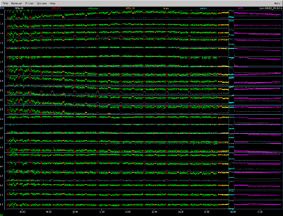
Background information about the observation In 2007 and 2009, the SMA (in subcompact configuration) did a line survey of the well known carbon star IRC+10216 (CW Leo). The results of the survey were published in Patel et al., 2011, ApJ Supp volume 193. The discussion below outlines the calibration of one track from that survey (data set 090202_07:19:01, taken on Feb. 2, 2009). Imaging is described in a separate section, "Imaging SMA Data with CASA". The plot to the right shows the corrPlotter display (a useful graphical summary) for this data set. Clicking on this (and other plots on this website) will bring up a new window, which can be expanded to full-screen for legibility. |
|
The script and caveats A script is available that calibrates and images the lower sideband of IRC+10216 (full description below and in "Imaging SMA Data with CASA" section of this website). The data was collected in "Double Bandwidth" mode (or single receiver, 4 GHz mode), which is by far the most common SMA observing mode. Because the 4 GHz IF is sent to the ASIC correlator via two independent IF pathways, the upper 2 GHz (chunks s25-s48) can drift in phase relative to the lower 2 GHz (chunks s01-s24). Many of the calibration steps are therefore performed on the two IFs separately. The script takes about 6.5 hours to run on the computer cfa0. Lines copied from the script (and other executable commands) appear in this font Before running the reduction script above, be sure to convert the data to CASA measurement set (MS) format:sma2casa.py -l -t See the "Python Scripts" section for details about sma2casa.py.Indentation is important in Python. It is used to determine the level of nesting in loops. Incorrect indentation can lead to unexpected results or failure to execute. Be careful when cutting and pasting. |
|
Basic definitions Define the waitForCASA() function: The waitForCASA() function is called between CASA tasks. It prevents CASA from starting a new task before the preceeding one has released its file locks.
Other definitions:
|
|
Import the data into CASA: Within CASA, type:
|
|
Create a "tiled" measurement set Issue the following commands:
Set the new value of vis:
|
|
Process the two IFs separately Issue the following commands, indented as shown:
|
|
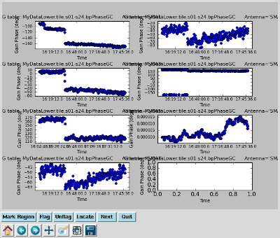
Phase-only gain calibration of bandpass calibrator During observation of the bandpass calibrator, 3C273, there were a couple of phase jumps and some phase drifting. In order to vector average these data, we first need to line up the phases. This is achieved by a phase-only gain calibration of 3C273 (essentially a self-calibration of the bandpass calibrator data). Issue the command, one line, indented:
Notes about parameter values:
|
|
Plot the gain calibration results Interrupt the script and issue the command, one line:
|
|
Solve for bandpass calibration table Issue the command, one line, indented;
Notes about parameter values:
|
|
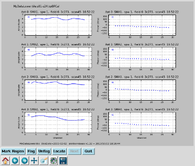
Plot the bandpass solution Interrupt the script and issue the command, one line (results to right):
|
|
Apply bandpass solution and derive short time scale phase only gain solutions Following the instructions on the NRAO SMA/CASA site, we apply the bandpass solution and derive a new short timescale phase-only gain solution for the bandpass calibrator. Issue the command, one line, indented:
|
|
Apply phase-only solutions and solve for longer timescale amplitude solutions Next, we apply the phase-only gain solutions and solve for longer timescale (solint) amplitude solutions to increase the S/N. Issue the command, one line, indented:
Note that in the command above, we are applying two gain tables. Since the second table was derived with a command which applied the first table, the effects of the two tables are cumulative. The spwmap parameter now has two items in its list, corresponding to the two gain tables. The first spwMap tells gaincal to apply the single phase gain calibration to all chunks being processed (remember we're processing chunks s01-s24 and s25-s48 separately) and the second argument tells gaincal to apply the bandpass solutions for chunk s{nn} to chunk s{nn}. |
|
Correct residual baseline-based problems after antenna-based bandpass calibration The SMA correlator often shows bandpass amplitude variations which are specific to particular baselines. These can only be corrected by a baseline-based (rather than antenna-based) bandpass calibration. This correction requires two steps (again, this is from the NRAO guide for reducing SMA data with CASA). The first step removes an overall normalization factor by combining all spws. Issue the command, one line, indented:
The second step does a baseline-based amplitude-only solution (per spw). Issue the command, one line, indented:
|
|
Set the flux scale Issue the command, indented:
This sets the flux of the gain calibrator, 0851+201. Note that only the first polarization flux (stokes I) is set. |
|
Final gain calibration of target (science) source Issue the command, one line, indented:
|
|
Apply calibration tables Issue the command, one line, indented:
This fills in the "corrected" data column in the MyDataLower.tile measurement set. |
|
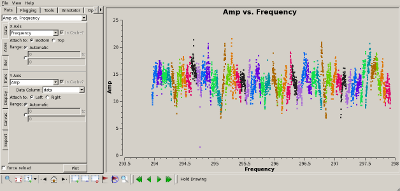
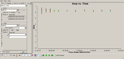
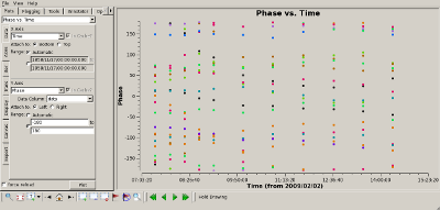
Check bandpass calibration Interrupt the script and use plotms(vis='MyDataLower.tile') to verify that the bandpass calibration flattened the phase and amplitude properly. The plots to the right show the amplitude (top) and phase (bottom) of the 3C273 data, for the "data" (uncalibrated) and "corrected" (calibrated) columns of the measurement set. |
 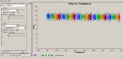 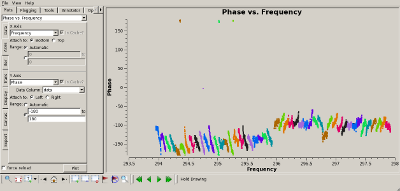 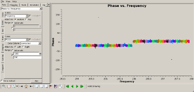
|
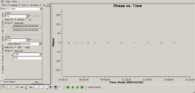
Check complex gain calibration Interrupt the script and use plotms() to show how well the complex gain calibration worked. The plots to the right show the amplitude (top) and phase (bottom) of the complex gain calibrator, 0851+202. All spws were averaged to produce these plots and all baselines are shown. The time average was set to 10 minutes, so that all integrations within a CASA scan would be summed to produce a single point. |
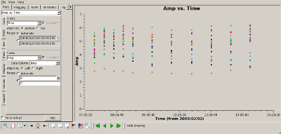   
|
Split off target data in preparation for imaging Since calibration is complete, calibrators are no longer necessary. Create a new measurement set with just the target source, IRC+10216:
The data are now ready for imaging (see the "Imaging SMA Data with CASA" section) |
| Commands | Plots |
|---|---|
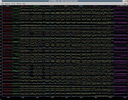
Background information about the observation In 2006, the SMA (in extended configuration) observed the CO(2-1) line in the Gomez Hamburger (IRAS 18059-3211), a pre main-sequence star. All 8 antennas were used. Most of the chunks were set to a coarse resolution of 32 channels/chunk, but several were set to 512 channels/chunk to target specific spectral lines. A single spectral line was detected, CO(2-1) in the USB of chunk s12, and the results were published in Bujarrabal et al., 2008, A&A 482, pp 839-845. The discussion below outlines the calibration of this source (data set 060609_07:34:16, taken on June 9, 2006). Imaging is described in a separate section, "Imaging SMA Data with CASA". The plot to the right shows the corrPlotter display (a useful graphical summary) for this data set. Clicking on this (and other plots on this website) will bring up a new window, which can be expanded to full-screen for legibility. |
|
The script and caveats A script is available that calibrates the upper sideband of the Gomez Hamburger data set (full description below). Lines copied from the script (and other executable commands) appear in this font Before running the calibration script above, be sure to convert the data to CASA measurement set (MS) format:sma2casa.py -u -t See the "Python Scripts" section for details about sma2casa.py.Indentation is important in Python. It is used to determine the level of nesting in loops. Incorrect indentation can lead to unexpected results or failure to execute. Be careful when cutting and pasting. |
|
Basic definitions Define the waitForCASA() function: The waitForCASA() function is called between CASA tasks. It prevents CASA from starting a new task before the preceeding one has released its file locks.
Define the "ones" array: The ones array (technically a Python list) is used later in the script to tell CASA to apply a single calibration to multiple SMA chunks (spws). The extra elements in the array (measurement set has only 24 spws) are not problematic.
|
|
Import the data into CASA: Within CASA, type:
execfile('smaImportFix.py')
|
|
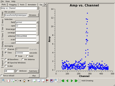
Plot the CO(2-1) line Interrupt the script and issue the command, one line (results to right):
|
|
Create a "tiled" measurement set Issue the commands (four lines):
Set the new value of vis:
|
|
Set the fluxes Issue the commands (five lines) to set the bandpass and gain calibrator fluxes:
The fluxdensity assignments come from the online SMA calibrator list. Even though this measurement set contains observations of Jupiter, Ganymede, and Uranus, it is too old for a standard flux calibration. The CASA ephemerides do not cover the 2006 observation date. Normally, one would do a primary flux calibration using Ganymede (and possibly Uranus), but in this case the CASA task that would bootstrap the calibration (setjy) does not work. |
|
Phase-only gain calibration of bandpass calibrator Issue the command, one line:
|
|
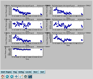
Plot the gain calibration results Interrupt the script and issue the command, one line (results to right):
|
|
Solve for bandpass calibration table Issue the command, one line;
Notes about parameter values:
|
|
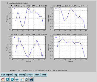
Plot the bandpass solutions Interrupt the script and issue the command (results on right):
|
|
Apply bandpass solution Issue the command:
|
|
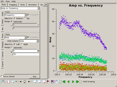
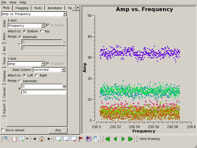
Check bandpass solution with plotms() Interrupt the script to check the bandpass calibration, for example, by plotting the amplitude of Uranus on the 1-* baseline. The results for the "raw" (uncalibrated) and "corrected" (calibrated) data columns are shown on the top right and bottom right, respectively. Clearly, the bandpass calibration has flattened the amplitudes. |
|
Gain calibration (phase and amplitude) Issue the command, one line:
|
|
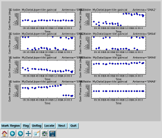
Plot gain calibration solutions Interrupt the script and issue the command, one line (results to right): plotcal(caltable='MyDataUpper.tile.gaincal',iteration='antenna',yaxis='phase',subplot=421,plotrange= [0,0,-180,180],overplot=True) |
|
Smooth calibration table The gain calibration plots (above) show that the phase calibration was noisy, particularly near the beginning of the track. Smooth the calibration table with the command, one line:
|
|
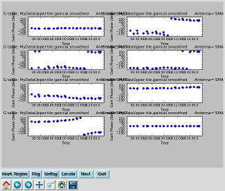
Plot smoothed gain calibration solutions Interrupt the script and issue the command, one line:
While the smoothed calibration table is indeed smoother, the solution still jumps around significantly early in the track. That's because two gain calibrators were used to derive the calibration table, and smoothcal can only smooth the solutions from the two sources separately. |
|
Apply bandpass and gain calibrations Apply the bandpass and gain calibration tables to the data, producing a "corrected" data column which can then be imaged. Issue the command, one line:
|
|
Split off target data in preparation for imaging Since calibration is complete, calibrators are no longer necessary. Create a new measurement set with just the target source:
Set the new value of vis in preparation for imaging:
The data are now ready for imaging (see the "Imaging SMA Data with CASA" section) |
| Commands | Plots |
|---|---|
|
This section assumes that the target source has been calibrated, either in CASA (see the "Calibrating SMA Data with CASA" section on this website), MIR, Miriad, or AIPS. Start imaging with the calibrated data file, "IRC10216_02Feb09_LSB_Calibrated". The imaging section of the IRC+10216 data reduction script starts with the first clean() command. |
|
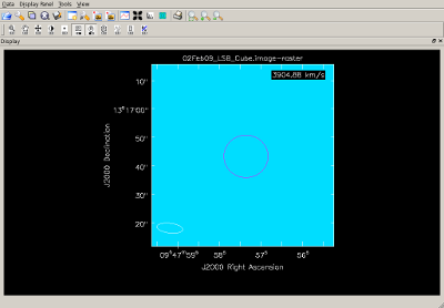
Prepare for continuum subtraction IRC+10216 has a continuum flux of about 1 Jy at 345 GHz and this must be subtracted from the data before final (line) image cubes are made. The steps for determining what parts of the spectrum to use for continuum subtraction are outlined below.
|
 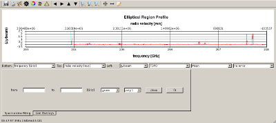 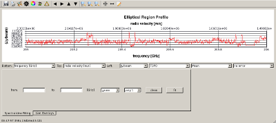 |
Subtract continuum from data using line-free regions determined above Type, one line:
|
|
Use continuum-free data to make a spectral cube Type, one line:
|
|
Use continuum-free data to map individual spectral lines Type, one line:
Type, one line:
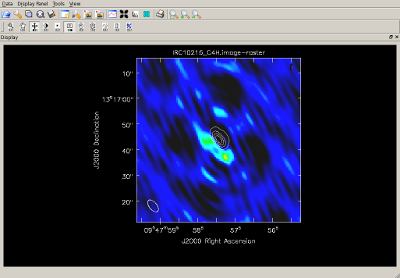
The image on the right shows a contour map of the SiCC line, along with a raster image of the C4H line. |
 |
| Commands | Plots |
|---|---|
|
This section assumes that the target source has been calibrated, either in CASA (see the "Calibrating SMA Data with CASA" section on this website), MIR, Miriad, or AIPS. The Gomez Hamburger data reduction script ends with the assignment, vis='gomezUSB'. This is the calibrated measurement set (MS) and will be used as the input to the clean commands below. If the calibration script was not run, enter the filename explicitly in the appropriate imaging commands. |
|
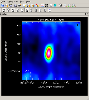
Image continuum and view the results It is clear from the corrPlotter display that continuum emission was detected from the science source. Image and view the upper sideband continuum emission, clean() on one line:
The resulting plot (right) shows that the source is slightly offset from phase center. |
|
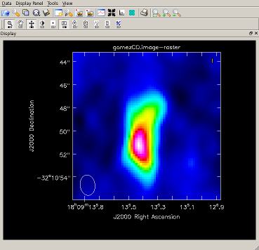
Image the CO Line and view the results The CO(2-1) line falls in the 22 channels of spw12 starting with channel 260 (plotms). Image and view, clean() on one line:
Clearly, the CO emission (right) is resolved. |
|
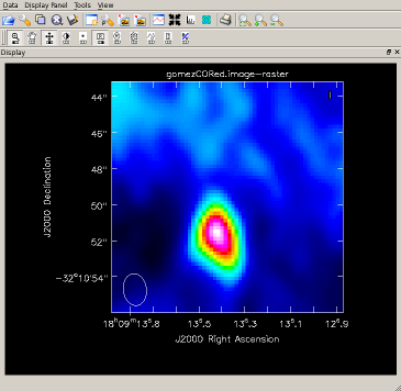
Image the red-shifted CO and view the results Image and view, clean() on one line (results to right):
|
|
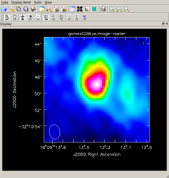
Image the blue-shifted CO and view the results Image and view, clean() on one line (results to right):
|
|
SMA CASA Issues
E-mail us at kyoung@cfa.harvard.edu and put the following in the subject line:
- "data" If related to computer access, running Python or CASA, etc.
- "website" if related to website viewing.
-
"mailing" if you wish to be added to our mailing list. Mailing list topics include:
- Notification of SMA CASA script updates
- Submitting error reports
- Tips, Shorts-Cuts, etc.
- Data testing and anaylsis
General CASA Information
Visit the National Radio Astronomy Observatory (NRAO) website, http://casa.nrao.edu.
