1. Selfcal for phase:
Task:   selfcal
  vis      = xmiriad050218_230_rx0.lsb
  select   = source(ti*,3c111*,ga*,ce*,17*)
  interval = .5
  refant   = 6
  offset   =
  line     = chan,1,1,3072
2. Start bee:
 Task:   bee
  vis      = miriad050128_230_rx0.lsb
  device   = /xs
Here are the interactive instruction for using the fitting, plotting and editting functions that are supported in bee:
Number of points= 130
Enter antenna to display : 1
Number of points= 130
AVAILABLE COMMANDS ARE:
1P   Fit axis offset
2P   2-parameter fit [sets B3 = -cotan(LAT)*B1]
3P   3-parameter fit to phase differences
4P   4-parameter fit; no 2PI discontinuities !
5P   5-parameter fit includes axis offset
AM   Plot amplitudes versus time
ED   Edit to new baseline etc.
EX   Exit BEE and write antpos file
FI   Seach for best fit baseline
GR   Plot vs. HA, sin(DEC), elevation, or focus
IN   Get the Gains for another antenna
LI   List antenna positions and current fit.
PH   Plot phase versus time
TE   Edit data to test fitting programs
TF   Tpower and Tair fit to phase
TH   Plot airtemp versus time
TP   Plot tpower versus phase and fit slope.
WA   Write ANTPOS file.
WG   Write gains into the output gains file.
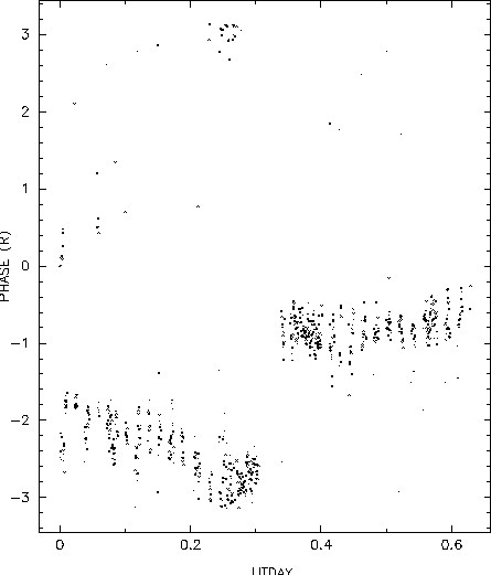
3. Plotting Phase:
One can use one of the commands, such as PH for plotting phase vs. time. Here is an exmaple:
command=ph
Plot phase versus time and fit.
SELECT SOURCES
Type source numbers separated by commas
<cr> means finished; <a> means all sources
   1  titan      2  3c111      3  ganymede   4  ceres
   5  1743-038
SOURCES: a
in plot window type
CURSOR OPTIONS:
A  restore deleted points
B  set bottom to cursor position
C  Connect cursor positions
D  move phase point down by 2pi
E  end manipulations on plot
F  show instrumental phase fit
G  fit gains to tpower plot
H  Hanning smooth fitted curve
I  Identify the sources
J  Join the plotted points
K  superpose temperature plot
L  set left to cursor position
M  plot more sources
N  set new limits and replot
O  superpose tpower plot
P  replot on printer
Q  position fit
R  set right to cursor position
S  replot
T  set top to cursor position
U  move phase point up by 2pi
V  delete point(s)
W  write the source labels at top of plot
X  average and rms of plotted points
0 - 8 order of polynomial fit
+  unwrap phase
 |
4. Baseline Fitting:
bee also supports least square fitting to the phase difference for new antenna positions:
command=in                                          % choose new antenna
Enter antenna to display :1                         % choose anetnna 1
 Number of points= 845
command=4p                                          % 4parameter fits
4-PARAMETER FIT
Fit antenna positions and constant phase offset
SELECT SOURCES
Type source numbers separated by commas
<cr> means finished; <a> means all sources
   1  titan      2  3c111      3  ganymede   4  ceres
   5  1743-038
SOURCES: a                                          % average all source
>>>> report of the results from the baseline fit to antenna 1 <<<<
  4 parameter fit, sigma:    0.0502
 initial baseline   14.80856 -213.06612  -72.84222    0.00000    0.00000
   new   baseline   14.81041 -213.06482  -72.84171   -2.24603    0.00000
  delta  baseline    0.00185    0.00130    0.00050   -2.24603    0.00000
  uncertainties     0.000017   0.000006   0.000011   0.008770
covariance matrix
       24.1681        0.1636        0.1474        0.9680
        0.0169       14.0156       -0.3741        0.0788
       -0.0087        0.0220        9.6160        0.2996
       -0.0259       -0.0021       -0.0080       29.5466
command=fi
Step size for bx/by/bz (    0.0020) :0.0001
# of steps in 1-D (       40.) :15
Step size for antmiss (    0.0020) :0.0001
# of steps (1=nofit) (        1.) :1
BEE FIT DATA--starting with:
bx =   14.8086  by = -213.0661  bz =-72.8422  antmiss = 0.0000  chisq =    3.09
bx =   14.8079  by = -213.0668  bz =-72.8429  antmiss = 0.0000  chisq =    1.63
bx =   14.8079  by = -213.0668  bz =-72.8428  antmiss = 0.0000  chisq =    1.63
bx =   14.8079  by = -213.0668  bz =-72.8427  antmiss = 0.0000  chisq =    1.63
bx =   14.8079  by = -213.0668  bz =-72.8424  antmiss = 0.0000  chisq =    1.62
bx =   14.8079  by = -213.0668  bz =-72.8423  antmiss = 0.0000  chisq =    1.62
bx =   14.8079  by = -213.0668  bz =-72.8422  antmiss = 0.0000  chisq =    1.53
bx =   14.8079  by = -213.0668  bz =-72.8421  antmiss = 0.0000  chisq =    1.45
bx =   14.8079  by = -213.0668  bz =-72.8420  antmiss = 0.0000  chisq =    1.44
bx =   14.8079  by = -213.0668  bz =-72.8419  antmiss = 0.0000  chisq =    1.44
bx =   14.8079  by = -213.0668  bz =-72.8416  antmiss = 0.0000  chisq =    1.39
bx =   14.8079  by = -213.0667  bz =-72.8426  antmiss = 0.0000  chisq =    1.32
bx =   14.8079  by = -213.0667  bz =-72.8425  antmiss = 0.0000  chisq =    1.32
bx =   14.8079  by = -213.0667  bz =-72.8416  antmiss = 0.0000  chisq =    1.19
bx =   14.8079  by = -213.0666  bz =-72.8416  antmiss = 0.0000  chisq =    1.10
bx =   14.8079  by = -213.0666  bz =-72.8415  antmiss = 0.0000  chisq =    1.10
bx =   14.8079  by = -213.0664  bz =-72.8419  antmiss = 0.0000  chisq =    1.02
bx =   14.8079  by = -213.0663  bz =-72.8417  antmiss = 0.0000  chisq =    1.01
bx =   14.8079  by = -213.0662  bz =-72.8418  antmiss = 0.0000  chisq =    1.01
bx =   14.8079  by = -213.0662  bz =-72.8417  antmiss = 0.0000  chisq =    1.01
bx =   14.8079  by = -213.0662  bz =-72.8416  antmiss = 0.0000  chisq =    1.01
bx =   14.8079  by = -213.0662  bz =-72.8415  antmiss = 0.0000  chisq =    1.01

command=in
Enter antenna to display :2                        % for antenna 2
 Number of points= 846
command=4p
4-PARAMETER FIT
Fit antenna positions and constant phase offset
SELECT SOURCES
Type source numbers separated by commas
<cr> means finished; <a> means all sources
   1  titan      2  3c111      3  ganymede   4  ceres
   5  1743-038
SOURCES: a
  4 parameter fit, sigma:    0.0131
 initial baseline  -19.01948  -63.32772   52.06702    0.00000    0.00000
   new   baseline  -19.01964  -63.32768   52.06705    0.60843    0.00000
  delta  baseline   -0.00015    0.00005    0.00004    0.60843    0.00000
  uncertainties     0.000005   0.000002   0.000003   0.002456
covariance matrix
       23.9466        0.2085        0.1593        0.9686
        0.0940       13.4426       -0.4154        0.1348
        0.0298       -0.0778        9.5842        0.3195
        0.0621        0.0086        0.0205       29.0861
command=fi
Step size for bx/by/bz (    0.0020) :0.0001
# of steps in 1-D (       40.) :15
Step size for antmiss (    0.0020) :0.0001
# of steps (1=nofit) (        1.) :1
BEE FIT DATA--starting with:
bx =  -19.0195  by =  -63.3277  bz = 52.0670  antmiss = 0.0000  chisq =    0.10
bx =  -19.0202  by =  -63.3278  bz = 52.0663  antmiss = 0.0000  chisq =    0.10
bx =  -19.0202  by =  -63.3277  bz = 52.0663  antmiss = 0.0000  chisq =    0.10
bx =  -19.0202  by =  -63.3276  bz = 52.0663  antmiss = 0.0000  chisq =    0.10
One can go through the least square fitting for all the antennas
to obtain corrections for positions.
The gains derived from amplitude and phase fits are write to the gains file and the new antenna position can be written out to a text file. Here is an exmaple:
command=EX

The gains derived from amplitude and phase fits
using the ED command are written at this time.
The gains are written into the output gains file.
The default output is the input uvdata file.

OK to write the gains ?y
Number of solution intervals: 875
5. Write New Antenna Positions:
Enter filename for antenna positions: antpos.new
#Fitted antenna positions - Mon Mar 21 16:25:18 2005
     14.8079   -213.0662    -72.8415
    -19.0202    -63.3276     52.0663
     -1.6940    -83.9048      4.2696
     17.4370    -66.9718    -49.5145
    -59.7692   -198.6647    100.2966
      0.0000      0.0000      0.0000
      0.0000      0.0000      0.0000
      0.0000      0.0000      0.0000