BANDPASS

Normally, an observation track includes a bandpass scan on a small planet or a strong quasar. As long as the visibility data on each channel gives adequate S/N, one can solve for antenna-based bandpass solutions using smamfcal. Here is an exmaple for solving for bandpass based on observations of the Jupiter's moon, Callisto.

  Task:   smamfcal
  vis      = gc_rx1.lsb.tsys % input data with Tsys correction 
                               and bad data that are flagged.
  select   = source(call*)   % here select a calibrator with 
                               wildcard call* = callisto
  refant   = 3
  interval = 100           % time interval for bandpass solutions
  weight   = 2             % the channel visibility is normalized
                           % by the average of channels specified
                           % by the inner 75% of each "spectral 
                             chunk";

The above setup of smamfcal for bandpass is given using the calibrator Callisto. The solutions can be checked with smagpplt:

smagpplt% inp
  Task:   smagpplt
  vis      = gc_rx1.lsb.tsys   % input file with bandpass table
  device   = /xs               % x-window device
  log      =                
  yaxis    = amp,phase         % displays amplitude and phase
  options  = bandpass,opolyfit % bandpass; bandpass solutions 
                                 will be replaced by the 
                                 polynomial fit
  polyfit  = 5                 % the 5th order polynomial is 
                                 used in the least square fit.
  nxy      = 2,4               % page setup: 2 in row and 4 in 
                                 column.

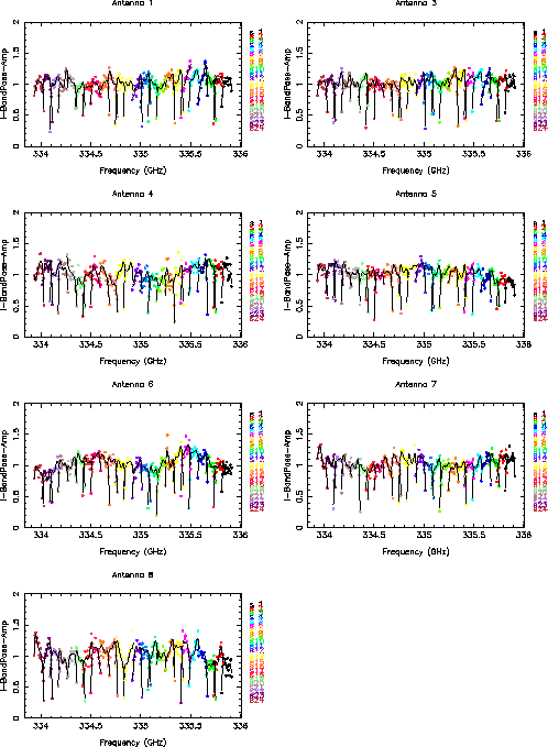
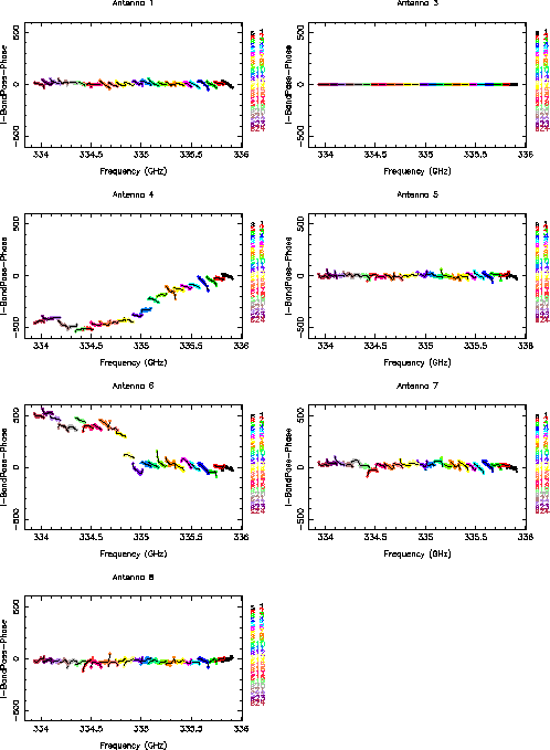
The solutions for amplitude and phase are shown in (Figs. 3.1 and 3.2). The ripples in amplitude shown in the antenna based solutions across the 2 GHz band needs to be corrected. The data of antenna 2 is relatively noisy and poor. Antenna 2 has been removed before solving for bandpass. Antenna 4 shows a large delay across all the chunks. Antenna 6 shows a big phase jump between the first 3 blocks (12 chunks) and the next 3 blocks. The phase solutions of the antennas are with respect to the reference antenna 3. The errors must be removed. This is particularly important for continuum data which is an average of the spectral data. Also the bandpass solution appears to be little noisy and one can fit a polynomial to the solutions. The solid curves are the fitted version of the bandpass solutions. If the polynomial fit is satified, one can run smagpplt by re-setting the options to options = bandpass,opolyfit with other parameters remaining the same. Then the bandpass solutions are replaced by the polynomial fit. Note that the options of opolyfit will replace the original solution. We encourage users to try these parameters. If mistakes occur, one can always re-run smamfcal to calculate the solutions again.

Figure: Bandpass solutions in amplitude. The solid black curves are the 5th polynomial fit to the solutions.

Figure: Bandpass solutions in phase. The solid black curves are the 5th polynomial fit to the solutions.