Flux calibration

The flux calibration is done with a set of IDL routines written by Tom Matheson. They are described at length in Sec. 2.2 of the reductio.ps file contained in the redux/ directory created during the installation process (see below). You are strongly advised to read this document as you go through the Step by step tutorial!

Installation

You will need both the redux and wombat packages, which you can download as tarballs locally at:

/data/www/projects/supernova/SNfast/redux.tar
/data/www/projects/supernova/SNfast/wombat.tar

Copy both tarballs to your IDL directory and unpack them there. This will create redux/ and wombat/ directories that contain all the IDL routines. Make sure these directories are in your IDL path, e.g.:

setenv IDL_STARTUP /home/username/idl/idl_startup.pro     [in your .cshrc]

where idl_startup.pro contains the following:

pathsep = path_sep(/search_path)
!path = expand_path('+/home/username/idl/') + pathsep + !path

Test data

In what follows we will go through one example of flux calibration on FAST spectra of supernovae. These data were taken on 29 Mar 2008 with the standard Combo setup (300 gpm grating and 3'' slit).

Start by copying the data over to a directory of your choice (hereafter called <REDUCE_DIR>):

~> cp /data/www/projects/supernova/SNfast/reduced/d*ms.fits <REDUCE_DIR>

These d*ms.fits files are the 1D wavelength-calibrated spectra extracted in multispec format using standard IRAF routines.

Go to <REDUCE_DIR> and create a file (here called dlist) containing the names of all the d*ms.fits files:

~> cd <REDUCE_DIR>
~> ls d*.ms.fits > dlist
~> cat dlist
d0107.HD84937.ms.fits
d0108.HD84937.ms.fits
d0109.HD84937.ms.fits
d0111.Feige34.ms.fits
d0117.sn2008bf.ms.fits
d0119.sn2008ax.ms.fits
d0121.sn2008bm.ms.fits

These files comprise spectra of two standard stars (three spectra of HD84937 and one spectrum of Feige34) and three supernova spectra.

IMPORTANT: Make sure the headers for these files have been corrected using the flwofixhead.cl IRAF script, as the IDL routines expect certain non-standard header keywords to be present. This is done automatically when reducing the data using the tasks presented in Spectral extraction and wavelength calibration. Refer to this webpage for more information on how to set up the flwofixhead.cl IRAF script (and similar scripts for data from other telescopes: flwofixhead.cl, kastfixhead.cl, lcofixhead.cl, lrisfixhead.cl, mmtfixhead.cl, oldkastfixhead.cl, ssofixhead.cl, uvfixhead.cl, vltfixhead.cl).

Then start idl in that same directory:

~> idl
IDL>

Step by step tutorial

Contents: Preamble | Making the Flux star | Flux Calibration | Making the B star | Final calibrations

NOTE: You can compare your output files at any stage of the tutorial with those located in /data/www/projects/supernova/SNfast/reduced/

0. Preamble

The main driver for the flux calibration is the cal.pro routine located in the redux/ directory. The syntax is as follows:

cal, second [, /fast]

where second is a positive integer that should be non-zero to enable second-order correction mode (in which case two standard stars are used instead of one). In this tutorial we will apply a second-order correction, so we should type the following command at the IDL prompt:

IDL> cal, 1

This will open up an IDL graphics terminal with the title Wombat. Feel free to resize this window.

NOTE on second-order correction: (taken from Tom Matheson's notes on "The Supernova Operation at Mt. Hopkins"): The wavelength range for the FAST includes the Balmer break, implying that a sdO star is the best calibrator. Recent improvements to the optics have enhanced the blue throughput, however, introducing a severe second-order light contamination. It is especially bad for a blue object like a sdO star. There is no perfect solution, but the best compromise is to use two standard stars with different colors. Calibrating the objects in the blue with the sdO star and in the red with a sdF star. This means that both a red and a blue standard should be observed every night. If this is not possible, the stability of FAST allows you to employ a standard from a nearby night. Here is a list of the good standards to use (note that other standards are observed with FAST--don't use them):
Star type Coords. (J2000.0) ---------------------------------------------- HD 19445 red 03:08:25.589 +26:19:51.39 HD 84937 red 09:48:56.100 +13:44:39.32 BD+26 2606 red 14:49:02.357 +25:42:09.16 BD+17 4708 red 22:11:31.374 +18:05:34.17 Hiltner 600 red 06 45 13.371 +02 08 14.70 Feige 34 blue 10:39:36.740 +43:06:09.25 BD+28 4211 blue 21:51:11.022 +28:51:50.36 Feige 110 blue 23:19:58.398 -05:09:56.21
NOTE on the /fast option: Running cal.pro with the /fast option (i.e. IDL> cal, 1, /fast) will tune the settings to those commonly used for SN spectral reductions with the FAST spectrograph. In this tutorial we will not use this option, but check out the various "NOTE on the /fast option" for more info. (Note that you should use this option when reducing FAST SN spectra for sake of consistency!)

You should see the following output on your screen:

% Compiled module: CAL.
 Welcome to cal.pro

This program is a driver for the calibration routines.
It expects files that have been dispersion calibrated,
usually through IRAF (you know, with a -d- in front).
(In other words, include the d in your file names.)


First, should this be an interactive or non-interactive
session?  Interactive sessions ask more questions so you
have more control, but take longer.

You have selected second-order correction mode

Interactive? (y/n)

Answering 'y' here will turn on the interactive mode for the four core routines (realmkfluxstar.pro, calibrate.pro, realmkbstar.pro, and final.pro; see below). You are stongly advised to use interactive mode!

NOTE on the /fast option: setting the /fast option will automatically select interactive mode.

You are then prompted to enter a "grating code":

Interactive? (y/n)
y

We now need a grating code, such as opt or ir2.
This will be used to keep track of the fluxstar and
bstar as in fluxstaropt.fits or bstarir2.fits

Enter the grating code:

You should enter a name that corresponds to the "blue" standard star (or to the single standard star if you haven't selected second-order correction mode). That name is used to generate various files along the way. Here our "blue" standard is Feige34, so let's pick f34b as our grating code ("f34" for "Feige34", with a "b" appended for "blue"; note that you can pick any name you want here):

Enter the grating code: f34b

You then need to enter the filename corresponding to the "blue" standard star:

Now the fits file for the fluxstar.

Fluxstar file:

Here we should enter the name of the 1D wavelength-calibrated extracted spectrum (in multispec format) corresponding to Feige34:

Fluxstar file: d0111.Feige34.ms.fits

Then comes this most obscure question:

Do you want to use the same star as the b-star? (y/n)

This simply means "do you want this same standard star spectrum to be used for removal of telluric features?", cf. the section below on Making the B-star spectrum. If the standard star spectrum has a flat continuum at the wavelengths of the atmospheric A- and B-bands (7620 A and 6880 A, respectively), as is the case here, answer 'y':

Do you want to use the same star as the b-star? (y/n)
y

Since we are running cal.pro with the second-order correction mode, the same set of questions is asked for the "red" standard star (HD84937 in our case):

Enter the grating code for the second standard: h84r

Now the fits file for the second fluxstar.

Fluxstar file: d0109.HD84937.ms.fits

Do you want to use the same star as the b-star? (y/n)
y

NOTE: There are three spectra available for HD84937. In general one should pick standard stars that were taken closest in airmass to the science targets. In our case, all spectra were taken at an airmass ≤ 1.1:
~> gethead d*ms.fits airmass d0107.HD84937.ms.fits 1.110352 d0108.HD84937.ms.fits 1.110944 d0109.HD84937.ms.fits 1.111565 d0111.Feige34.ms.fits 1.027796 d0117.sn2008bf.ms.fits 1.027708 d0119.sn2008ax.ms.fits 1.018854 d0121.sn2008bm.ms.fits 1.075248
so any HD84937 spectrum will do here.

NOTE on the /fast option: setting the /fast option will select grating codes and corresponding spectra. However, this option requires the presence of a file named std.list in the working directory. This file contains the names of the standard stars, one per line ("blue" standard first!). In our case this file will look like:
~> cat std.list Feige34 HD84937
Check out lines 118-130 in cal.pro for the list of available standard star names and corresponding grating codes (more can be added if necessary).

Next we need to specify the name of the file containing the list of spectral filenames (dlist in our case):

Now for the file containing the list of objects.

Object list file: dlist

OK, here we go.

We are now ready to make the flux stars (see below).

1. Making the Flux star (`realmkfluxstar.pro`)

The first core routine called by cal.pro is realmkfluxstar.pro, with which the continuum of the standard star(s) is fit and saved away as a fits file fluxstar<GRATING_CODE>.fits (i.e. fluxstarf34b.fits and fluxstarh84r.fits in our example). See Sec. 2.2.1 of the reductio.ps file contained in the redux/ directory created during the installation process.

The syntax of realmkfluxstar.pro is as follows:

realmkfluxstar, fluxfile, gratcode, intera [, /fast]

In our current example, this routine is automatically called by cal.pro as: (again starting with the "blue" standard star)

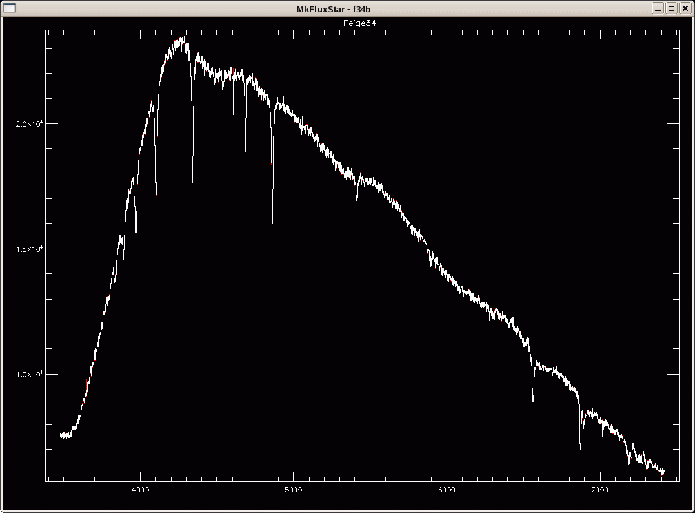
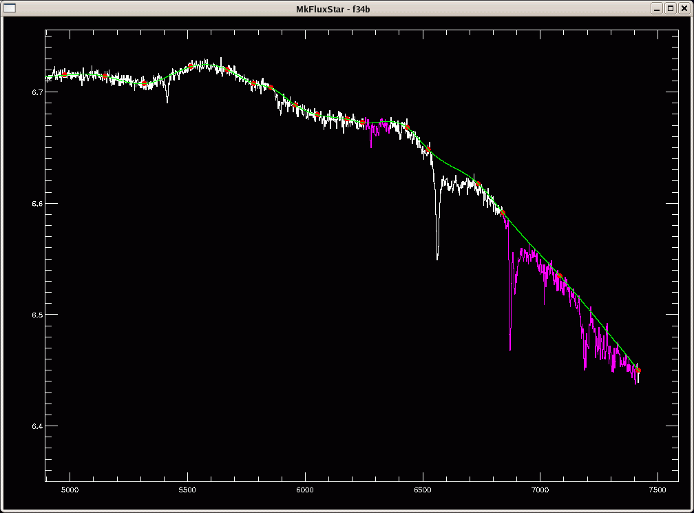
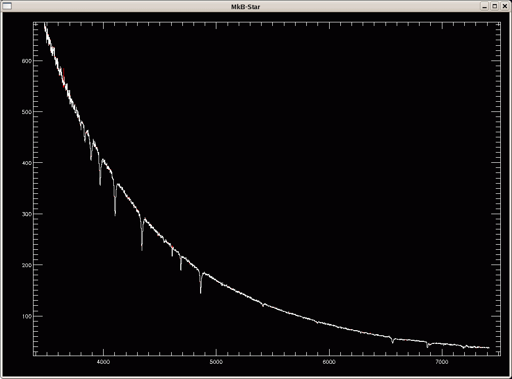
realmkfluxstar, 'd0111.Feige34.ms.fits', 'f34b', 1

The "blue" standard star is plotted up in the graphics output terminal (normal extraction in red, optimal in white). Click on the thumbnail below to see the result:

The user is prompted for which extraction to use; you should chose the optimal extraction (by typing 'o') unless you have good reasons not to do so:

Flux star routine
% Compiled module: REALMKFLUXSTAR.
% Compiled module: READFITS.
% Compiled module: SXPAR.
% Compiled module: GETTOK.
% Compiled module: VALID_NUM.
% READFITS: Now reading 2683 by 1 by 4 array
% Compiled module: PACHECK.
% Compiled module: SXADDPAR.
     120
% Compiled module: GETMSWAVE.
% Compiled module: FINALSCALER.
Plotting optimal as white, normal as red
Do you want to use the (n)ormal or the (o)ptimal extraction?
o

You then have to select which star your "blue" standard corresponds to from a long list. In our case the "blue" standard is (27) FEIGE 34 (STONE):

% Compiled module: QUADTERP.
% Compiled module: ZPARCHECK.
% Compiled module: ABCALC.
The object is Feige34

  WHICH STANDARD STAR IS THIS ?
  ORIGINAL MCSP FLUX STANDARDS (AB79 SCALE):
  (1) HD 19445       (2) HD 84937        (3) BD+262606
  (4) BD+17 4708       (5) HD 140283 (SOMEWHAT OBSOLETE)
  OTHERS (AB69, AB79, STONE, OR BALDWIN/STONE SCALE):
  (6) GD-248 (AB79)            (7) G158-100 (AB79)
  (8) LTT 1788 (B/S)           (9) LTT 377 (B/S)
  (10) HZ 4 (~AB79)            (11) HZ 7 (~AB79)
  (12) ROSS 627 (~AB79)        (13) LDS 235B (~AB79)
  (14) G99-37 (~AB79)          (15) LB 227 (~AB79)
  (16) L745-46A (~AB79)        (17) FEIGE 24 (~AB79)
  (18) G60-54 (~AB79)          (19) G24-9 (AB79)
  (20) BD+28 4211 (STONE)      (21) G191B2B (~AB79)
  (22) G157-34 (AB79)          (23) G138-31 (AB79)
  (24) HZ 44 (~AB79)           (25) LTT 9491 (B/S)
  (26) FEIGE 110 (STONE)       (27) FEIGE 34 (STONE)
  (28) LTT 1020 (B/S)          (29) LTT 9239 (B/S)
  (30) HILTNER 600 (STONE)     (31) BD+25 3941 (STONE)
  (32) BD+33 2642 (STONE)      (33) FEIGE 56 (STONE)
  (34) G193-74 (AB79)          (35) EG145 (OKE,74)
  (36) FEIGE 25 (STONE)        (37) PG0823+546
  (38) HD 217086               (39) HZ 14
  (40) FEIGE 66                (41) Feige 67 (Groot special)
  (42) LTT 377                 (43) LTT 2415
  (44) LTT 4364                (45) Feige 15
  (46) Hiltner 102 (lousy)     (47) LTT 3864
  (48) LTT 3218                (49) CYG OB2
  (50) VMa 2                   (51) EG 274 (Hamuy)
  (52) LTT 3218 (Hamuy)        (53) LTT 6248 (Hamuy)
  (54) LTT 7987 (Hamuy)        (55) L870-2
  (56) CD 32                   (57) LTT 4816
  (58) EG 131
: 27

Now you need to manually fit a spline to the continuum of the blue standard star (this is the most time-consuming part of the flux calibration).

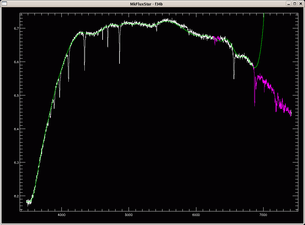
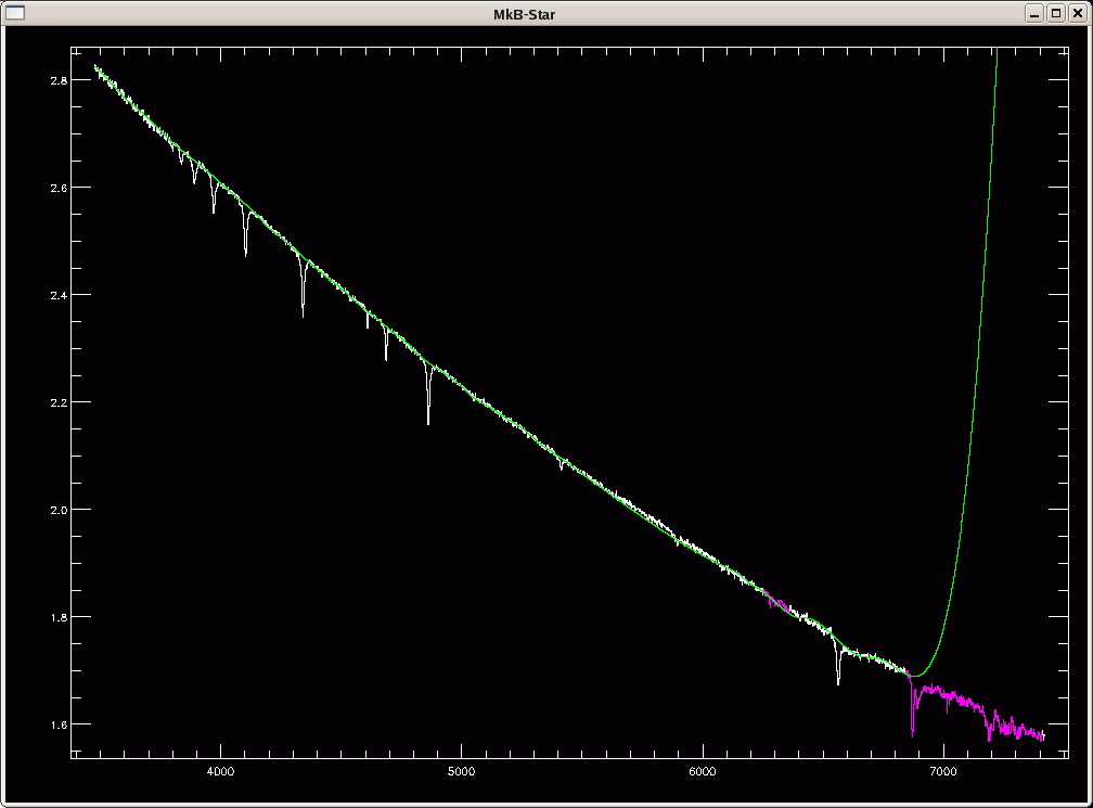
The star is plotted in white, atmospheric and stellar absorption bands are purple, and the spline is green. Click on the thumbnail below to see the result:

The user is asked whether this is OK, which it obviously is not (and will never be the way the routine is currently written) for this first automatic try:

Time to fit the continuum manually.

% Compiled module: FITSPLINE.
% Compiled module: GET_ELEMENT.
% Compiled module: UNIQ.
% Compiled module: INT.
% Compiled module: SIGN.
% Compiled module: CAST.
% Compiled module: TYPE.
% Compiled module: DEFAULT.
Is this ok? (y/n)

If you answer 'n', you will be asked whether you want to change the plot scale, which enables you to zoom in on certain parts of the spectrum. I typically answer 'y' here, and then you can mark the lower-left and upper-right corners of the zoom region with the left mouse button:

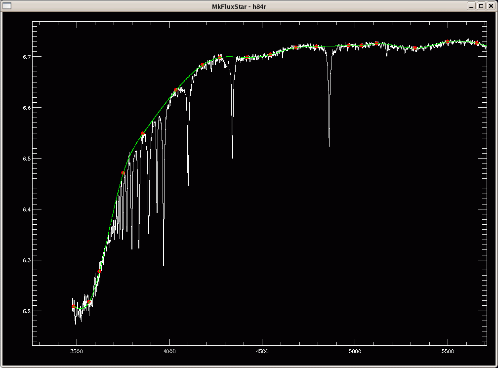
Change scale? (y/n)

  Mark the corners of your box...

Click on the thumbnail below to see the result of zooming in on the blue part of the spectrum:

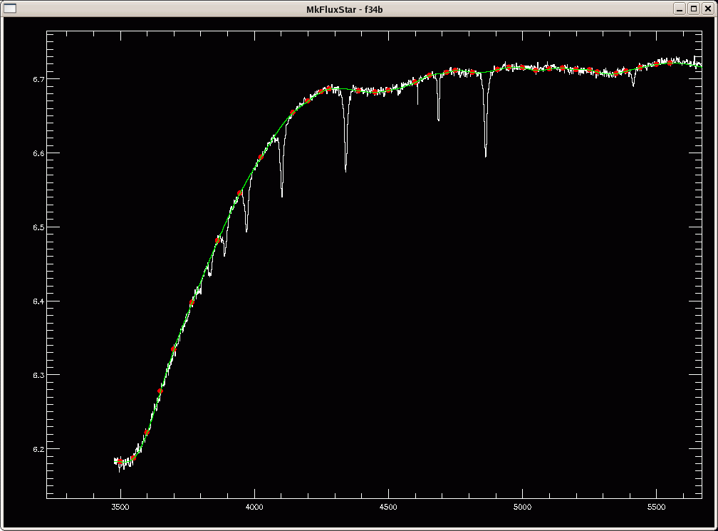
The spline knot points are plotted in red, and you can add points, delete the point nearest to the cursor, and (re)fit a spline by moving the cursor with the mouse and with the 'a', 'd', and 'f' keyboard keys:

Select continuum points for spline fit (up to 500).
(a)dd point
(d)elete point
(f)it spline

NOTE: If you'd rather use mouse buttons instead of keyboard keys to add points, delete the point nearest to the cursor, and (re)fit a spline, you can uncomment lines 315-361 in the fitspline.pro routine. You would then see the following message:
Click on continuum points for spline fit (up to 500). Left button = add point Middle button = delete point Right button = done
You can iterate back and forth, constantly redrawing the fit so that it is clear. A good rule to follow is to fit to the white part, and to make a smooth curve (the true stellar continuum) over the purple parts. Another thing is to make sure the ends of the spline don't do anything crazy. We don't trust the data out there anyway, but it can give enormous flux values to spurious data, and this makes it hard to see the whole spectrum later on when it is scaled to the crazy data in final.pro (see Final calibrations).

Once you're satisfied with the spline fit, hit the 'f' key once more, then answer 'n' to the Is this ok? (y/n) query (since we still need to fit the red part of the spectrum!), then 'y' to change the scale and zoom in on the red portion of the spectrum.

Click on the thumbnails below to see a satisfactory to the blue part of the spectrum (left); a satisfactory to the red part of the spectrum (middle); and the fit to the overall spectrum (right):

Now answering 'y' to the Is this ok? (y/n) query will create the flux star file fluxstarf34b.fits:

Is this ok? (y/n)
% Compiled module: SXDELPAR.
Writing data to fluxstarf34b.fits
% Compiled module: WRITEFITS.
% Compiled module: CHECK_FITS.
% Compiled module: FXPAR.
% Compiled module: FXADDPAR.
% CHECK_FITS: NAXIS keywords in FITS header have been updated
% CHECK_FITS: BITPIX value of -64 added to FITS header

NOTE on the /fast option: setting the /fast option will automatically chose the optimal extraction, and select the number in the standard star list corresponding to the flux star spectrum.

Since we are running cal.pro with the second-order correction mode, the same set of operations needs to be done for the "red" standard star:

Second flux star routine
% READFITS: Now reading 2683 by 1 by 4 array
      12
Plotting optimal as white, normal as red
Do you want to use the (n)ormal or the (o)ptimal extraction?
o
The object is HD84937

  WHICH STANDARD STAR IS THIS ?
  ORIGINAL MCSP FLUX STANDARDS (AB79 SCALE):
  (1) HD 19445       (2) HD 84937        (3) BD+262606
  (4) BD+17 4708       (5) HD 140283 (SOMEWHAT OBSOLETE)
  OTHERS (AB69, AB79, STONE, OR BALDWIN/STONE SCALE):
  (6) GD-248 (AB79)            (7) G158-100 (AB79)
  (8) LTT 1788 (B/S)           (9) LTT 377 (B/S)
  (10) HZ 4 (~AB79)            (11) HZ 7 (~AB79)
  (12) ROSS 627 (~AB79)        (13) LDS 235B (~AB79)
  (14) G99-37 (~AB79)          (15) LB 227 (~AB79)
  (16) L745-46A (~AB79)        (17) FEIGE 24 (~AB79)
  (18) G60-54 (~AB79)          (19) G24-9 (AB79)
  (20) BD+28 4211 (STONE)      (21) G191B2B (~AB79)
  (22) G157-34 (AB79)          (23) G138-31 (AB79)
  (24) HZ 44 (~AB79)           (25) LTT 9491 (B/S)
  (26) FEIGE 110 (STONE)       (27) FEIGE 34 (STONE)
  (28) LTT 1020 (B/S)          (29) LTT 9239 (B/S)
  (30) HILTNER 600 (STONE)     (31) BD+25 3941 (STONE)
  (32) BD+33 2642 (STONE)      (33) FEIGE 56 (STONE)
  (34) G193-74 (AB79)          (35) EG145 (OKE,74)
  (36) FEIGE 25 (STONE)        (37) PG0823+546
  (38) HD 217086               (39) HZ 14
  (40) FEIGE 66                (41) Feige 67 (Groot special)
  (42) LTT 377                 (43) LTT 2415
  (44) LTT 4364                (45) Feige 15
  (46) Hiltner 102 (lousy)     (47) LTT 3864
  (48) LTT 3218                (49) CYG OB2
  (50) VMa 2                   (51) EG 274 (Hamuy)
  (52) LTT 3218 (Hamuy)        (53) LTT 6248 (Hamuy)
  (54) LTT 7987 (Hamuy)        (55) L870-2
  (56) CD 32                   (57) LTT 4816
  (58) EG 131
: 2
Time to fit the continuum manually.

Is this ok? (y/n)
Change scale? (y/n)

  Mark the corners of your box...
Select continuum points for spline fit (up to 500).
(a)dd point
(d)elete point
(f)it spline

Is this ok? (y/n)
Writing data to fluxstarh84r.fits
% CHECK_FITS: NAXIS keywords in FITS header have been updated
% CHECK_FITS: BITPIX value of -64 added to FITS header

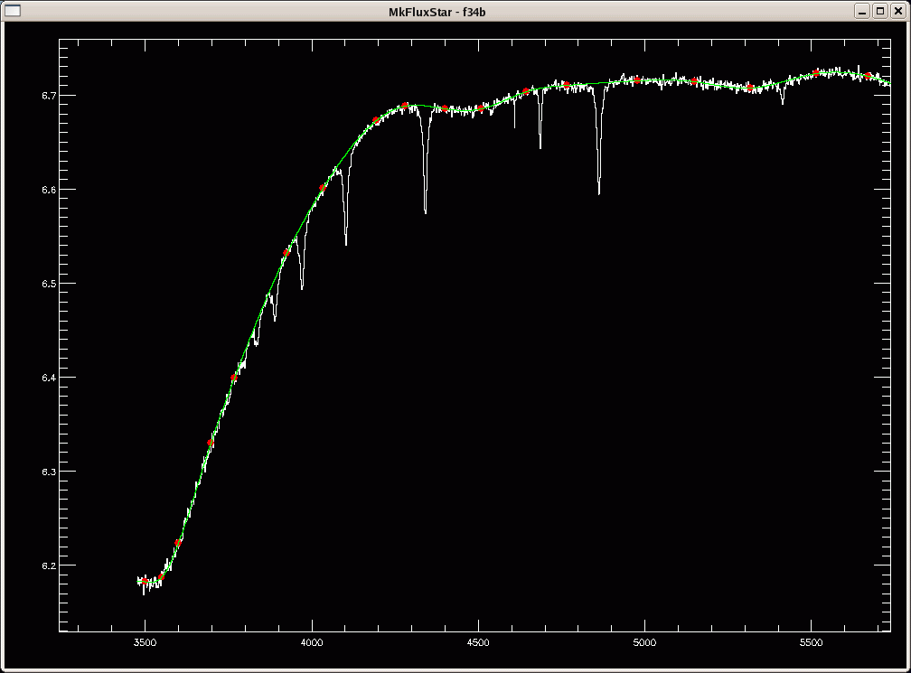
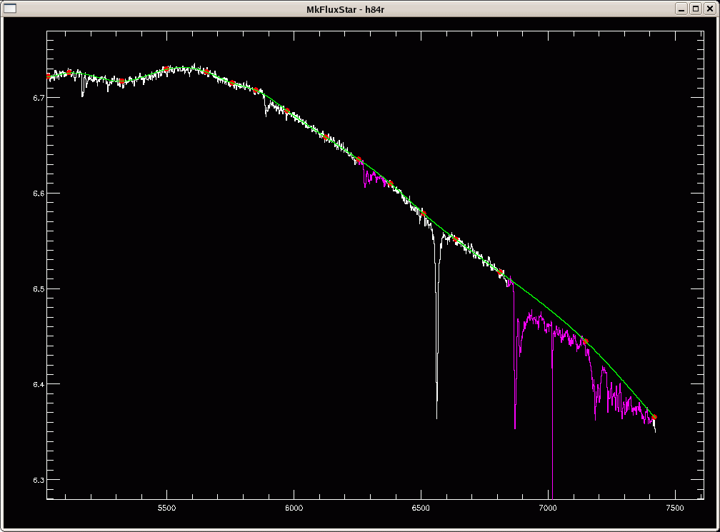
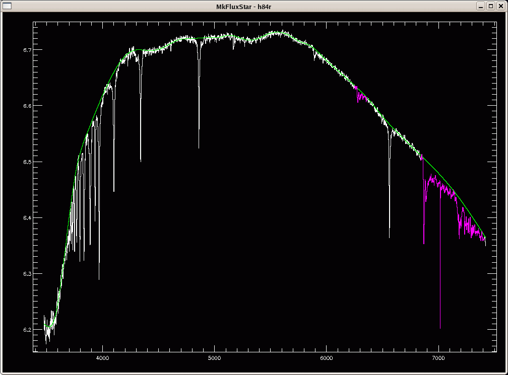
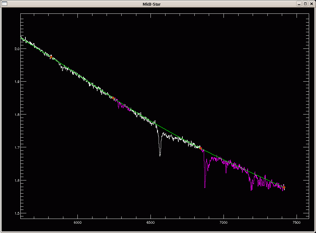
Again, you can click on the thumbnails below to see a satisfactory to the blue part of the spectrum (left); a satisfactory to the red part of the spectrum (middle); and the fit to the overall spectrum (right):

You can see that there is some ambiguity in defining the stellar continuum in the blue part of the spectrum of HD84937 (blueward of the Balmer 4000 A break), but we need not to worry since we will be using the blue standard star Feige34 to calibrate that part of the spectrum (see Final calibrations).

Now we have the two flux star files fluxstarf34b.fits and fluxstarh84r.fits. We will use these to calibrate our 1D spectra. This is done with the calibrate.pro task described below.

2. Flux calibration (`calibrate.pro`)

The second core routine called by cal.pro is calibrate.pro, with which the spectra are flux calibrated.

The syntax of calibrate.pro is as follows:

calibrate, infile, gratcode, intera, second, gratcode2

The "infile" is the file containing the list of spectral filenames (dlist in our case). The "gratcode" is the grating code for the blue standard ('f34b' here), and "intera" should be set to a strictly positive integer for interactive mode. "second" should also be set to a strictly positive integer if in second-order correction mode, in which case "gratcode2" is the grating code for the red standard ('h84r' here).

The output from this routine is a set of files named according to c<GRATING_CODE><FILENAME>.fits, where <GRATING_CODE> is one of "gratcode" or "gratcode2" and <FILENAME> corresponds to the files listed in the "infile".

In our current example, this routine is automatically called by cal.pro as:

calibrate, 'dlist', 'f34b', 1, 1, 'h84r'

which produces the following terminal output:

Calibration
% Compiled module: CALIBRATE.
% READFITS: Now reading 2683 array
% READFITS: Now reading 2683 array
% READFITS: Now reading 2683 by 1 by 4 array
The object is HD84937
Aperture 1:
% Compiled module: WOMIDLTERP.
% Compiled module: INTERPOL.
% CHECK_FITS: BITPIX value of -64 added to FITS header
% CHECK_FITS: BITPIX value of -64 added to FITS header
% READFITS: Now reading 2683 by 1 by 4 array
The object is HD84937
Aperture 1:
% CHECK_FITS: BITPIX value of -64 added to FITS header
% CHECK_FITS: BITPIX value of -64 added to FITS header
% READFITS: Now reading 2683 by 1 by 4 array
The object is HD84937
Aperture 1:
% CHECK_FITS: BITPIX value of -64 added to FITS header
% CHECK_FITS: BITPIX value of -64 added to FITS header
% READFITS: Now reading 2683 by 1 by 4 array
The object is Feige34
Aperture 1:
% CHECK_FITS: BITPIX value of -64 added to FITS header
% CHECK_FITS: BITPIX value of -64 added to FITS header
% READFITS: Now reading 2683 by 1 by 4 array
The object is sn2008bf
Aperture 1:
% CHECK_FITS: BITPIX value of -64 added to FITS header
% CHECK_FITS: BITPIX value of -64 added to FITS header
% READFITS: Now reading 2683 by 1 by 4 array
The object is sn2008ax
Aperture 1:
% CHECK_FITS: BITPIX value of -64 added to FITS header
% CHECK_FITS: BITPIX value of -64 added to FITS header
% READFITS: Now reading 2683 by 1 by 4 array
The object is sn2008bm
Aperture 1:
% CHECK_FITS: BITPIX value of -64 added to FITS header
% CHECK_FITS: BITPIX value of -64 added to FITS header

and creates the following files:

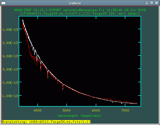
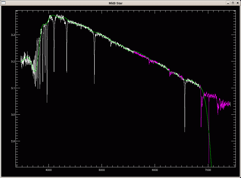
~> ls c*ms.fits
cf34bd0107.HD84937.ms.fits   ch84rd0107.HD84937.ms.fits
cf34bd0108.HD84937.ms.fits   ch84rd0108.HD84937.ms.fits
cf34bd0109.HD84937.ms.fits   ch84rd0109.HD84937.ms.fits
cf34bd0111.Feige34.ms.fits   ch84rd0111.Feige34.ms.fits
cf34bd0117.sn2008bf.ms.fits  ch84rd0117.sn2008bf.ms.fits
cf34bd0119.sn2008ax.ms.fits  ch84rd0119.sn2008ax.ms.fits
cf34bd0121.sn2008bm.ms.fits  ch84rd0121.sn2008bm.ms.fits

For example, cf34bd0111.Feige34.ms.fits is the Feige34 spectrum calibrated by itself, while ch84rd0111.Feige34.ms.fits is the same spectrum calibrated using the HD84937 flux star file. Note the difference between the two spectra in the plot below (click to enlarge), especially blueward of 4000 A! (the first spectrum is in white; the second in red).

NOTE: If you have fluxstar*.fits files from another night you'd like to use to flux calibrate a particular set of spectra, you can run calibrate.pro directly without starting cal.pro. In that case, you simply need to make a list of all 1D wavelength-calibrated extracted spectra (e.g., in a file called dlist) and run calibrate.pro as (assuming the flux star files are called fluxstarf34b.fits and fluxstarh84r.fits):
IDL> calibrate, 'dlist', 'f34b', 1, 1, 'h84r'
In that case, you will also need to run final.pro as a standalone routine (see Final calibrations).

3. Making the B star (`realmkbstar.pro`)

The third core routine called by cal.pro is realmkbstar.pro, the purpose of which is to create normalized spectra from the standard stars only including telluric features. The output is saved away as a fits file bstar<GRATING_CODE>.fits (i.e. bstarf34b.fits and bstarh84r.fits in our example). See Sec. 2.2.2 of the reductio.ps file contained in the redux/ directory created during the installation process.

The syntax of realmkbstar.pro is as follows:

realmkbstar, infile, gratcode, intera [, /fast]

In our current example, this routine is automatically called by cal.pro as: (again starting with the "blue" standard star)

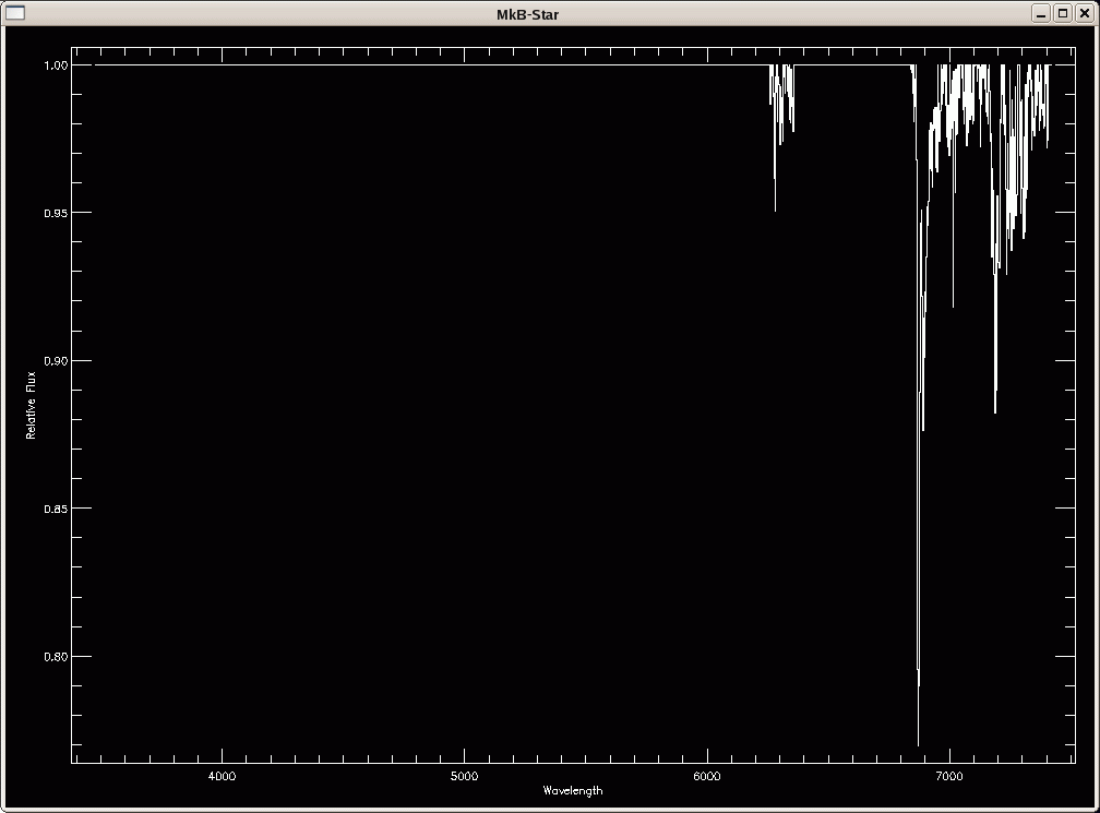
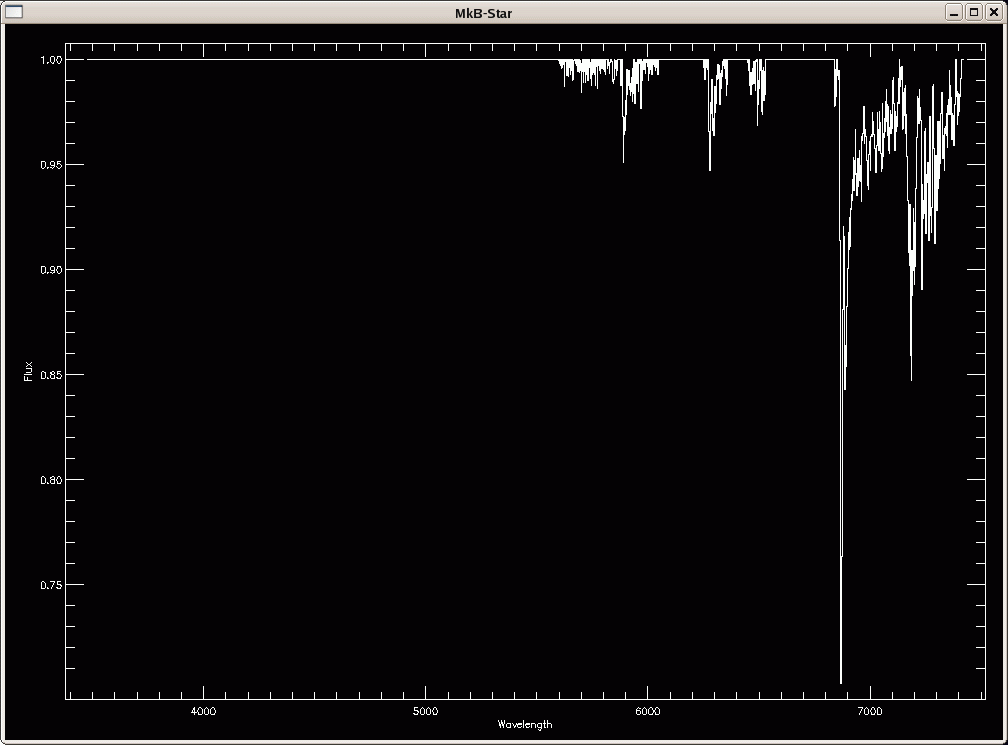
realmkbstar, 'cf34bd0111.Feige34.ms.fits', 'f34b', 'y'

NOTE: The "infile" here is the blue standard star spectrum calibrated by itself (see plot below). This makes it easier to fit the continuum on either side of prominent telluric features. Also note that for some reason the "intera" argument is now a string ('y' or 'n') as opposed to an integer.

The user is (again) prompted for which extraction to use; you should chose the optimal extraction (by typing 'o') unless you have good reasons not to do so:

B-star routine
% Compiled module: REALMKBSTAR.
% READFITS: Now reading 2683 by 1 by 4 array
% Compiled module: AVG.
Plotting optimal as white, normal as red
Do you want to use the (n)ormal or the (o)ptimal extraction?
o

The value of the AIRMASS keyword in the fits header is then displayed, and the user is asked to chose an airmass limit above which the airmass is considered "high" (we enter 1.1 in the example below to correct for weaker atmospheric bands; see the NOTE on the airmass limit):

Airmass =        1.0277960

Above what airmass is considered high? 1.1

In non-interactive mode this limit is set to 1.5.

NOTE on the airmass limit: (taken from Sec. 2.2.2 of the reductio.ps file contained in the redux/ directory): The regions of the spectrum that are adjusted by the B-star are as follows:
Range (A) Source Identifier ------------------------------------------- 3000-3190 O_3 Huggins 3216-3420 O_3 Huggins 5600-6050 (*) H_2O --- 6250-6360 O_2 --- 6450-6530 (*) H_2O --- 6840-7410 O_2(+H_2O) B(+alpha)-band 7560-8410 O_2(+H_2O) A(+z)-band 8800-9900 H_2O gamma & rho-bands (*) High airmass, sec z ≥ 1.5
Under certain circumstances, namely extremely high signal-to-noise ratio observations, the high-airmass water bands will appear even at low airmass. (This is most easily observable in the band-head at 6515 A.) To correct this, there is an interactive version of realmkbstar.pro that allows the user to set the airmass at which the weaker bands are corrected. If you want to correct for these weaker bands, just set the limit to something less than the B-star airmass.

The next step is to fit the continuum, in the same spirit as it was done for the flux star (see Making the Flux star). The star is plotted in white, atmospheric absorption bands are purple, and the spline is green. Click on the thumbnail below to see the result:

Since the airmass limit we chose (1.1) is greater than the airmass at which the Feige34 spectrum was taken, only the stronger atmospheric absorption bands are plotted in purple. We can zoom in on that (red) portion of the spectrum to fit the continuum around these features. This is done in exactly the same way as for the flux star routine (see Making the Flux star), except that we only need to ensure the spline fit is satisfactory in the purple regions (the B star spectrum is set to 1 at all other wavelengths).

Time to fit the B-star continuum manually.

Is this ok? (y/n)
Change scale? (y/n)
Select continuum points for spline fit (up to 500).
(a)dd point
(d)elete point
(f)it spline

       5477.4738       1.4437443
Is this ok? (y/n)

Click on the thumbnails below to see a zoom in on the red part of the spectrum, including a satisfactory spline fit, and the resulting normalized spectrum (right):

You are then asked whether you want to mask out some portions of the normalized B-star spectrum (e.g. sharp noise spikes). We do not need to do it here, but will do so for the second B star (see below). The output is then written as bstarf34b.fits.

Do you want to blotch the b-star (y/n, default=n)?
n
Writing data to bstarf34b.fits
% CHECK_FITS: NAXIS keywords in FITS header have been updated

Since we are running cal.pro with the second-order correction mode, the same set of operations needs to be done for the "red" standard star:

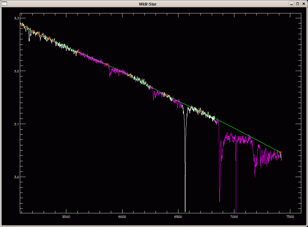
Second B-star routine
% READFITS: Now reading 2683 by 1 by 4 array
Plotting optimal as white, normal as red
Do you want to use the (n)ormal or the (o)ptimal extraction?
o

Airmass =        1.1115650

Above what airmass is considered high? 1.1
Time to fit the B-star continuum manually.

Is this ok? (y/n)
Change scale? (y/n)

  Mark the corners of your box...
Select continuum points for spline fit (up to 500).
(a)dd point
(d)elete point
(f)it spline
Is this ok? (y/n)

Here our chosen airmass limit of 1.1 is less that the airmass of the spectrum, and so the weaker atmospheric absorption bands are highlighted in purple (see plot below):

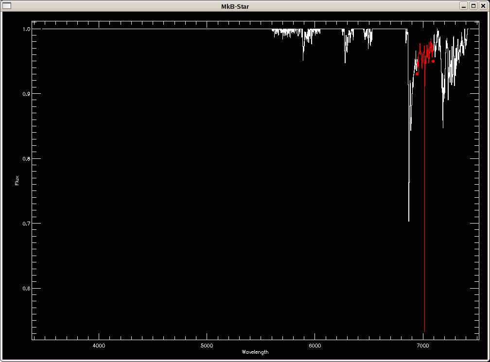
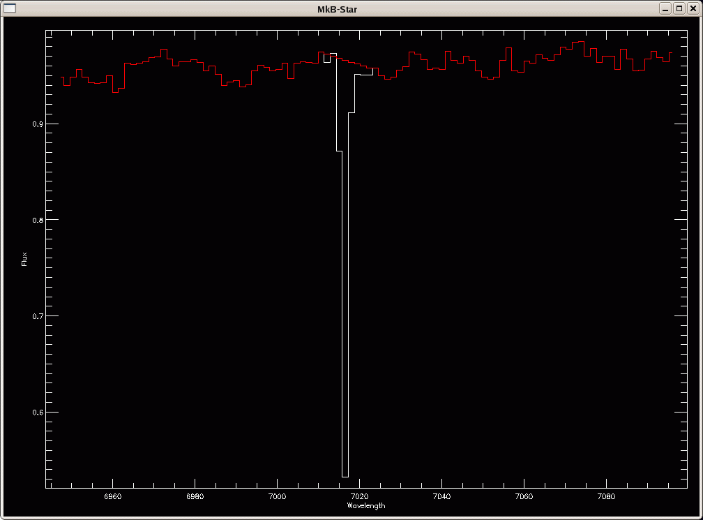
Click on the thumbnails below to see a zoom in on the red part of the spectrum, including a satisfactory spline fit, and the resulting normalized spectrum (right):

Notice the large negative noise spike (highlighted in red in the normalized spectrum). We will want to mask this out, and hence answer 'y' to the following question:

Do you want to blotch the b-star (y/n, default=n)?
y
% Compiled module: BBLO.
Select regions to blotch

% Compiled module: WOMWAVERANGE.

We can then zoom in on the region with the noise feature to blotch (here we select this zoomed wavelength range with the mouse by typing 'm'). The region is highlighted in red (as in the plot of the normalized spectrum above) and the user is asked to confirm the choice:

Do you want to select wavelength range by
entering (w)avelengths or marking with the (m)ouse? (w/m)
m

Spectrum runs from 3476.6941 to 7420.9327.

Mark the two end points of the region
       6947.8159      0.93004597
       7096.3679      0.94952248
Range selected: 6947.3887 to 7095.9227
Is this range correct? (y/n, default y)
y

The zoom region is plotted in the graphics terminal, and the user can select the bounds of the blotch region (in the example below with the mouse by typing 'm').

Do you want to enter blotch wavelengths by hand (w)
mark points (m), fit a spline (s), or quit (q) ?
m
Mark the two end points of the blotch region
       7012.3311      0.96511189
       7022.5025      0.95930190
Is this acceptable? (y/n, default=y)
y
Do another region? (y/n, default=n)
n
Writing data to bstarhd84r.fits
% CHECK_FITS: NAXIS keywords in FITS header have been updated

Click on the thumbnails below to see a zoom in on the blotch region with the blotched spectrum overplotted in red (right), and the resulting normalized spectrum, saved as bstarhd84r.fits.

Now that we have the two B-star spectra, we can proceed to the final calibration step.

NOTE on the /fast option: setting the /fast option will automatically chose the optimal extraction, and set the airmass limit to 1.1.

4. Final calibrations (`final.pro`)

The fourth and final core routine called by cal.pro is final.pro, which performs telluric feature removal, wavelength adjustments etc. on all the spectra listed in dlist (or whichever filename you chose). See Sec. 2.2.3 of the reductio.ps file contained in the redux/ directory created during the installation process.

The syntax of final.pro is as follows:

final, inputfile, gratcode, intera, secondord, gratcode2 [, /fast]

In our current example, this routine is automatically called by cal.pro as:

final, 'dlist', 'f34b', 1, 1, 'h84r'

NOTE: If you have fluxstar*.fits and bstar*.fits files from another night, you can run the above command directly (after having executed calibrate.pro) without starting cal.pro.

The final.pro routine then loops over the spectra (and each aperture within each extracted spectrum) listed in dlist, the first of which is a spectrum of HD84937 (d0107.HD84937.ms.fits).

First of all, final.pro asks the user to chose between the "optimal" and "normal" extractions, and then determines a heliocentric correction (here -20.9 km/s):

Final calibration (atmos. removal, sky line wave. adjust, etc.)
% Compiled module: FINAL.
% READFITS: Now reading 2683 array
% READFITS: Now reading 2683 array
% READFITS: Now reading 3395 array

Hello, sblondin
% READFITS: Now reading 2683 by 1 by 4 array
% READFITS: Now reading 2683 by 1 by 4 array
The object is HD84937
% Compiled module: GET_COORDS.
% Compiled module: TEN.
    2008       3      30       6       1       20.000000
% Compiled module: JDCNV.
% Compiled module: BARYVEL.
% Compiled module: PREMAT.

The velocity of the Earth toward the target is -20.903974 km/s.


There are 1 apertures in this spectrum.


Aperture 1:
% Compiled module: MOMENT.
Plotting optimal as white, normal as red
Do you want to use the (n)ormal or the (o)ptimal extraction?
o

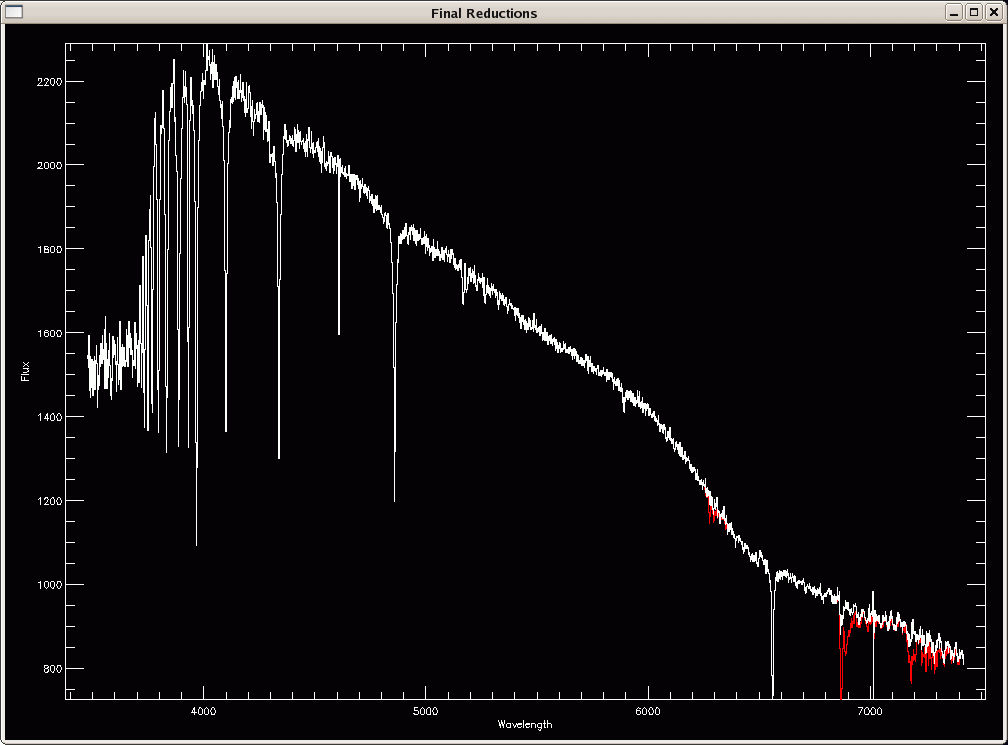
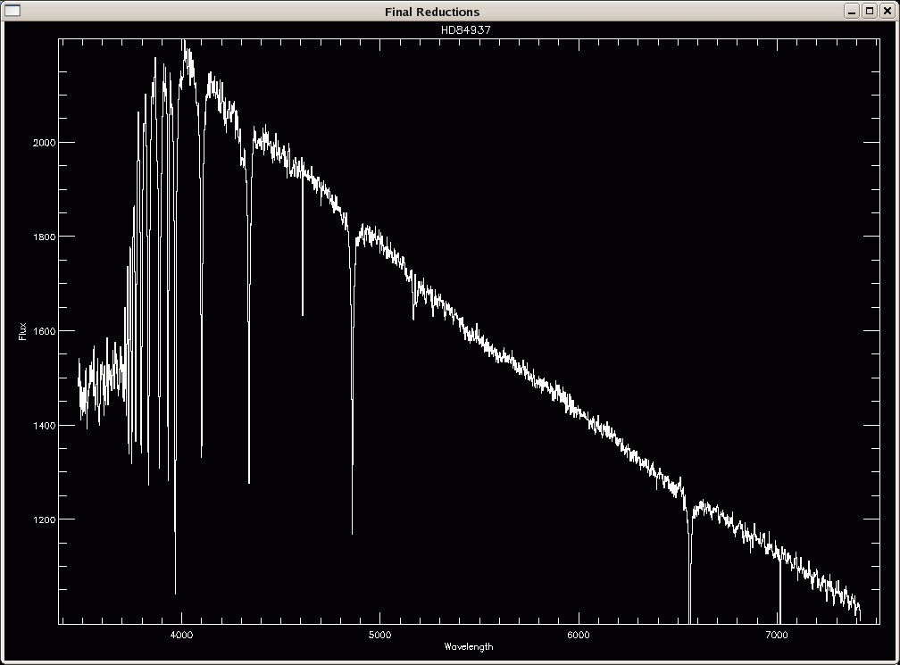
You can see a plot of the HD84937 spectrum below:

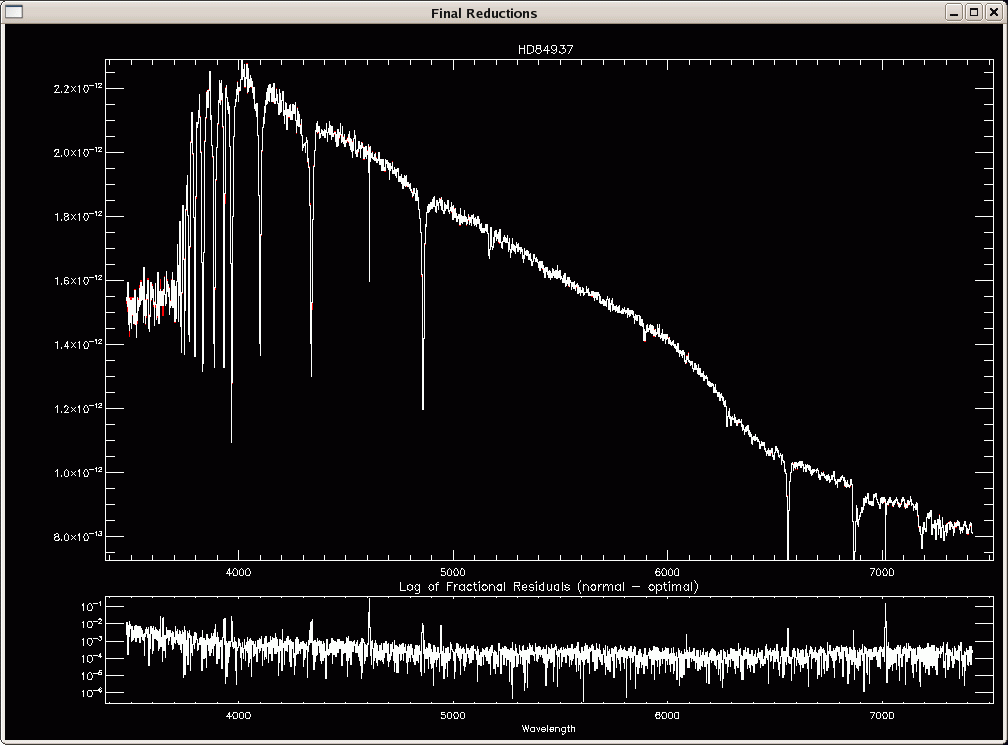
The spectral flux values are then scaled by a factor 1e15, and the extracted sky spectrum (in red below) is then cross-correlated with a master sky spectrum (in white below) for a final wavelength adjustment:

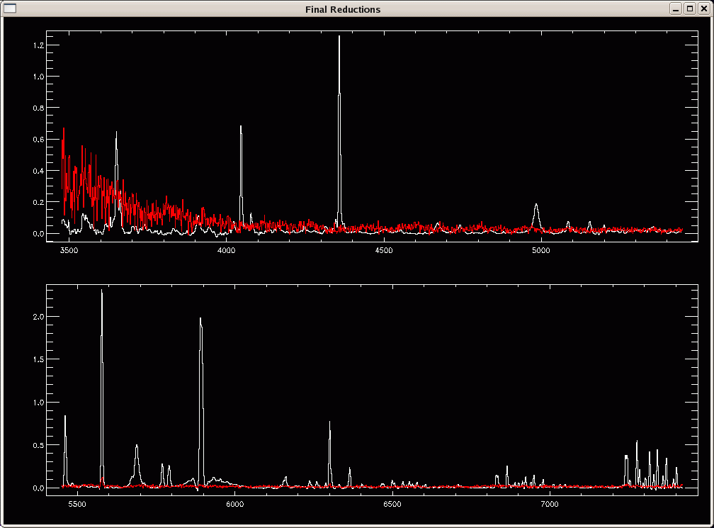
Scaling data up by a factor of 10^15...
The x-cor shift in Angstroms is       0.29412667

White spectrum = master sky
Red spectrum   = object sky shifted to match master sky
Is this ok (y/n, default=y)?

Since the exposure time for the HD84937 spectrum is only 12s, the sky lines are far from prominent. Nonetheless, the weak OI line at 5577 A matches that of the master sky spectrum, and the small correction of 0.29 A can be applied here, so we answer 'y' (if not, then you can specify the wavelength shift you want to apply, including 0 A).

Is this ok (y/n, default=y)? y

Removing redshift due to motion of the Earth...

The heliocentric correction is applied after this wavelength adjustment.

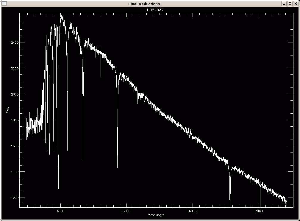
The next step is the removal of atmospheric absorption features using the B-star spectra. These are cross-correlated with the object spectrum at the B-band and the A-band. It determines a wavelength shift at each band, and averages them if both bands are in the spectrum:

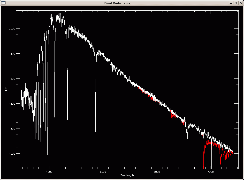
% Compiled module: TELLURIC_REMOVE.

The ratio of airmasses (object/B-star) is        1.0803233.

Cross-correlating object with B-star spectrum...

The shift at the B band is             2.4999023 Angstroms.
The mean shift is                      2.4999023 Angstroms.

Plotting spectrum before and after atmospheric band correction...
Is this ok? (y/n, default=y)

The ratio of airmasses (object/B-star) is       0.99890875.

Cross-correlating object with B-star spectrum...

The shift at the B band is             1.1764246 Angstroms.
The mean shift is                      1.1764246 Angstroms.

Plotting spectrum before and after atmospheric band correction...
Is this ok? (y/n, default=y)

You can see the result of applying this correction using the bstarf34b.fits and bstarh84r.fits B-star spectra below:

The result shown on the left (i.e. the HD84937 spectrum corrected using the bstarf34b.fits B star) is far less satisfactory than the one shown on the right (i.e. the HD84937 spectrum corrected using the bstarh84r.fits B star). This is OK, since we will use the "red" standard star (namely HD84937) to calibrate the red portion of our spectra (see below).

NOTE on the atmospheric feature removal: (taken from Sec. 2.2.3 of the reductio.ps file contained in the redux/ directory): If the removal does not look right, you can feed it whatever shift you want. When it doesn't look good there are several values to experiment with. First, if the B- and A-bands give very different values, try the value of each separately instead of the average. Often, zero is actually the best choice. If none of these work, you can iterate through as many shifts as you like, but keep in mind that the A-band is sometimes impossible to fix.

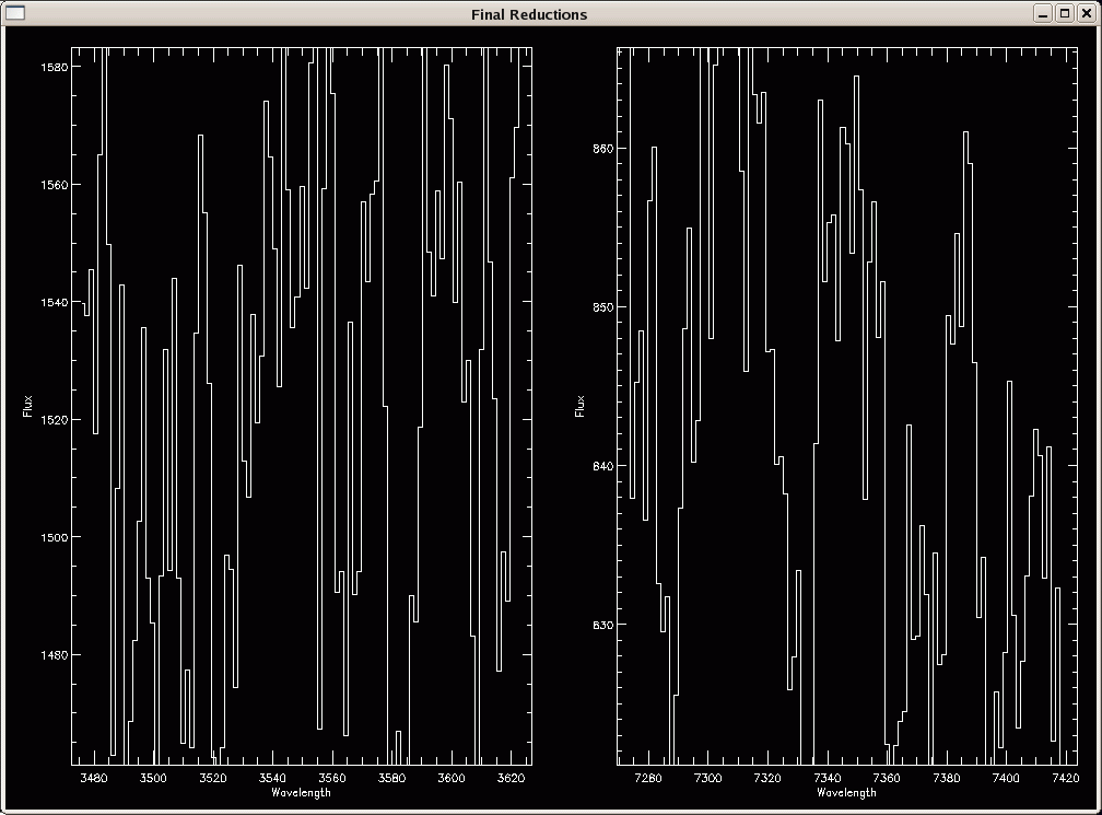
Next the two ends of the spectra are plotted (see plot below) and you can input a rebinning wavelength scale and endpoints (in the example below we accept the defaults by hitting <CR>):

Current A/pix is 1.4705308

Rebinning to  1.47 A. OK? [y/n; default=y]
OK, rebinning to  1.47 A.
newdelt =  1.47

Current range: 3476.1576 7420.1212

New suggested wavelength range is:  3477.00 7420

 Is this OK? [n/y; default=y]
NON-INTEGER number of bins

Closest match is:
       3477.0000        7421.0100
Would you like this wavelength range? (y/n, default=y)
y

This next step only applies to the second-order correction mode, which is the case here. The idea is to use the blue part (meaning blueward of the Balmer break) of the blue standard star spectrum to calibrate the blue portion of the spectra. Same line of argument for the red portion. The routine called is secondcat.pro.

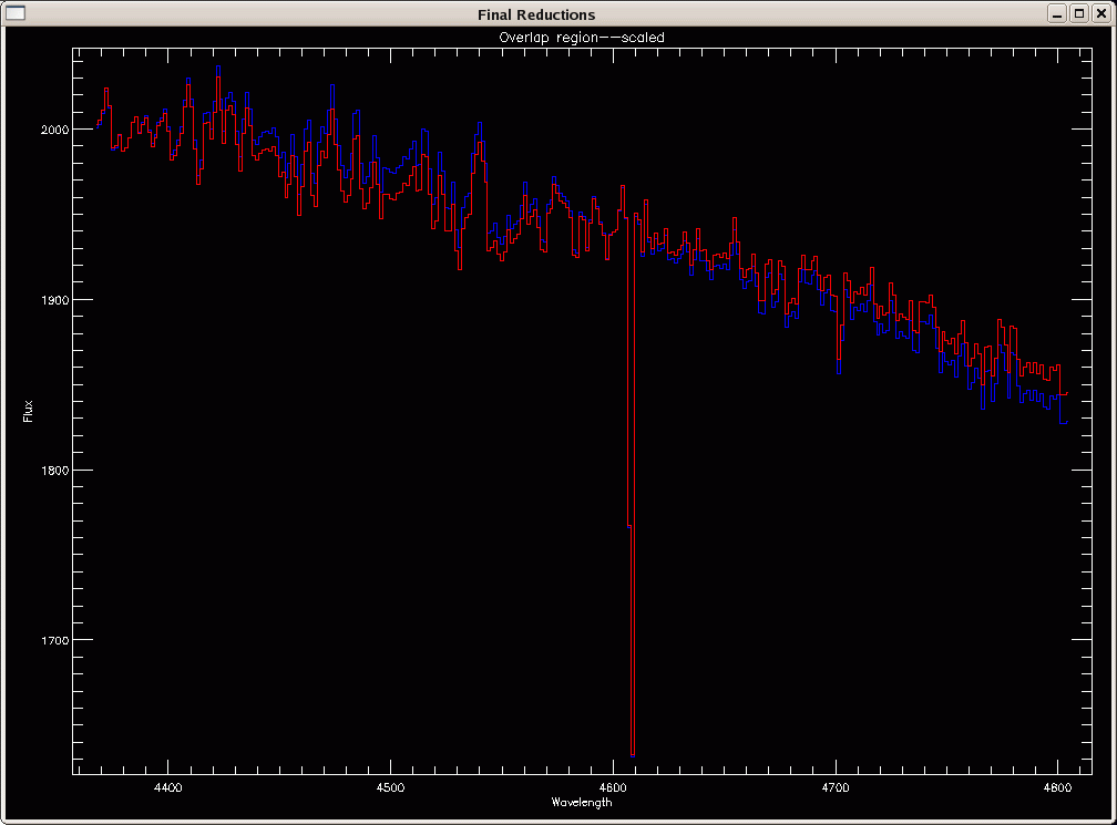
The user first has to select a range over which to an average flux value is used to scale the two spectra (i.e. a given spectrum calibrated using the blue standard, and that same spectrum calibrated using the red standard). You should usually pick a ~4300-4700 A range to compute the average (4368-4804 A below), i.e. slightly redward of the Balmer break. See the plot below:

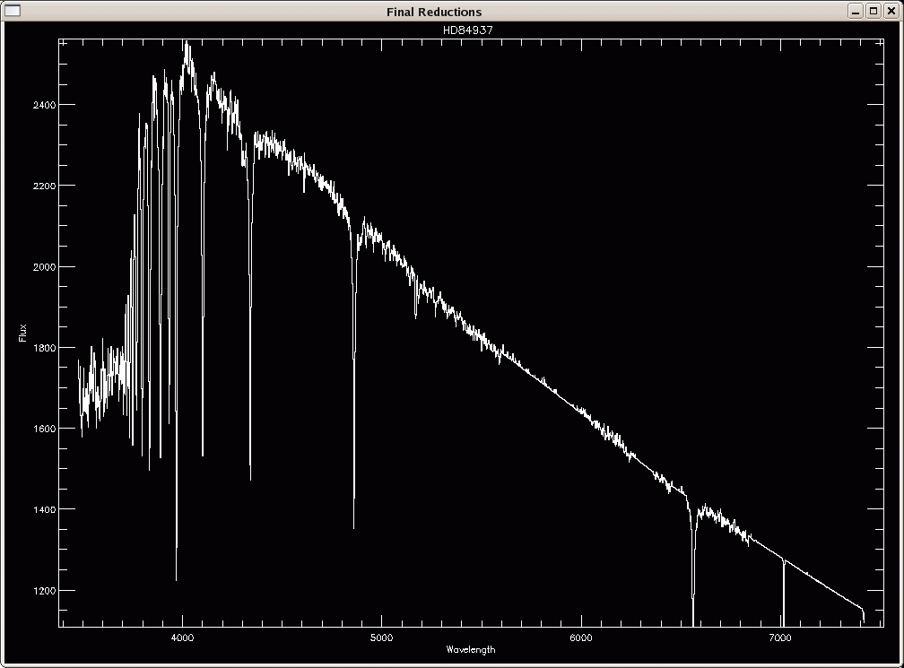
Combining two calibrated spectra:
Plotting blue side as blue, red side as red

Change y-scale? (y/n, default=n)
n
Mark the two end points of the region to compute average
       4368.3344       2008.9856
       4804.7993       1869.5640
Are these points ok? (y/n, default=y)
y
Average for range 4367.8200 to 4804.4100

Average for 4367.8200: 4804.4100
Blue side: 1995.0804
Red side: 1937.5141


Scale to blue or red? (b/r)
r
scale to red by 0.97114587

Note that scaling to the blue or red spectrum is up to you. Here we chose to scale to the red spectrum because HD84937 is our red standard star. You should check that the scale factor is close to unity (here it's 0.97).

Next we need to select a more restricted range over which the spectra will be combined. Blueward of this range, the blue standard star will be used to calibrate the spectrum; redward of this range, the red standard star will be used to calibrate the spectrum; within this range, a combination of the blue/red standards is used. In the example below we will combine the spectra over the range ~4450-4550 A (see plot below):

Plotting blue side as blue, red side as red

Change y-scale? (y/n, default=n)
n
Mark the two end points of the region to combine
       4450.5798       2036.4501
       4551.7310       2033.1986
Are these points ok? (y/n, default=y)
y
Combining over range 4450.1400 to 4551.5700

We're almost done! The final spectrum is plotted (see below), and you will be prompted for the object name. The output fits file will be called <OBJECT_NAME>-<UT-DATE>.fits, and the corresponding error spectrum will be saved as <OBJECT_NAME>-<UT-DATE>-sigma.fits.

The file is cf34bd0107.HD84937.ms.fits
The object is HD84937
The DATE-OBS is 2008-03-30
The aperture is 1
Previous name was
Enter the object name for the final fits file:
Object name is: HD84937
(UT date and .fits will be added): HD84937-a
% CHECK_FITS: NAXIS keywords in FITS header have been updated
% CHECK_FITS: BITPIX value of -32 added to FITS header
% CHECK_FITS: BITPIX value of -64 added to FITS header

Since there are several (three) spectra of HD84937, we append a -a to the object name. The output files are then HD84937-a-20080330.fits and HD84937-a-20080330-sigma.fits.

Several non-standard keywords are added to the fits header, listed below:

Keyword       Explanation
-------------------------
W_RANGE       wavelength range (A)
BSTAR_Z       airmass of B-star
BSTARNUM      file number of B-star
BSTAROBJ      name of B-star       
BARYVEL       velocity of the Earth toward the target (km/s)
SKYSHIFT      wavelength shift applied from cross-correlation with a master sky spectrum
ATMSHIFT      wavelength shift at position of the B- (and A- when present) atmospheric bands
EXTRACT       'optimal' or 'normal'
REDUCER       username of reducer
RED_DATE      epoch of reduction
OBJECT        user-defined object name
-------------------------
the keywords listed below are only 
for second-order correction mode
-------------------------
SECOND        'yes' if second order correction attempted
COMBRANG      range over which the blue and red spectra were combined (A)
BSTAR_Z2      airmass of 2nd B-star    
BSTARNU2      file number of 2nd B-star
BSTAROB2      name of 2nd B-star       
FLX2_Z        airmass of 2nd flux star 
FLX2_NUM      file number of 2nd flux star
FLX2_OBJ      name of 2nd flux star

The same process is repeated (apart from the selection of average and combine regions for the second-order correction, which is kept identical to the previous selection). You can see the terminal output for all other files: final_other.txt.

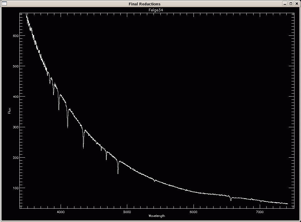
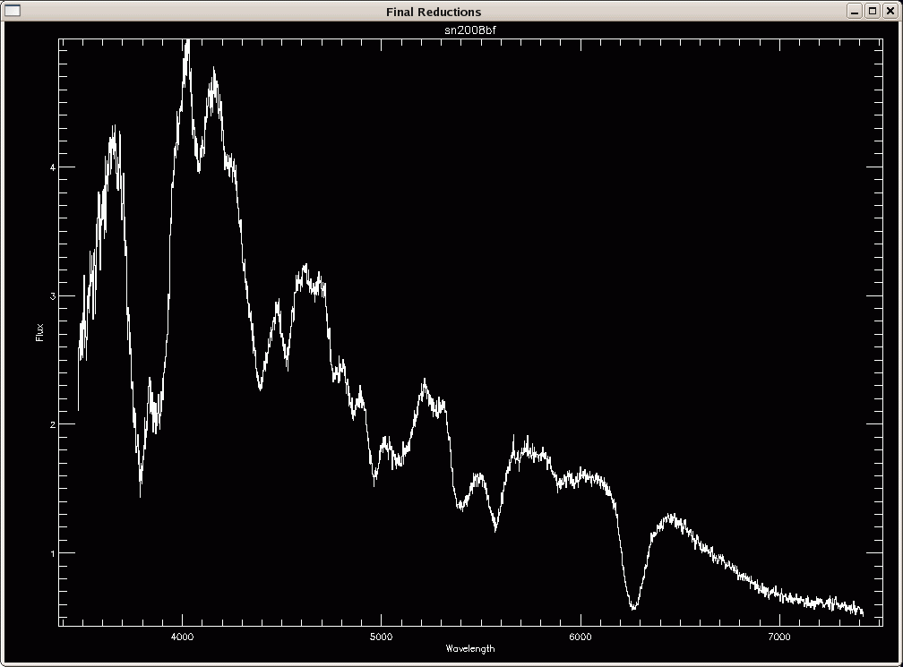
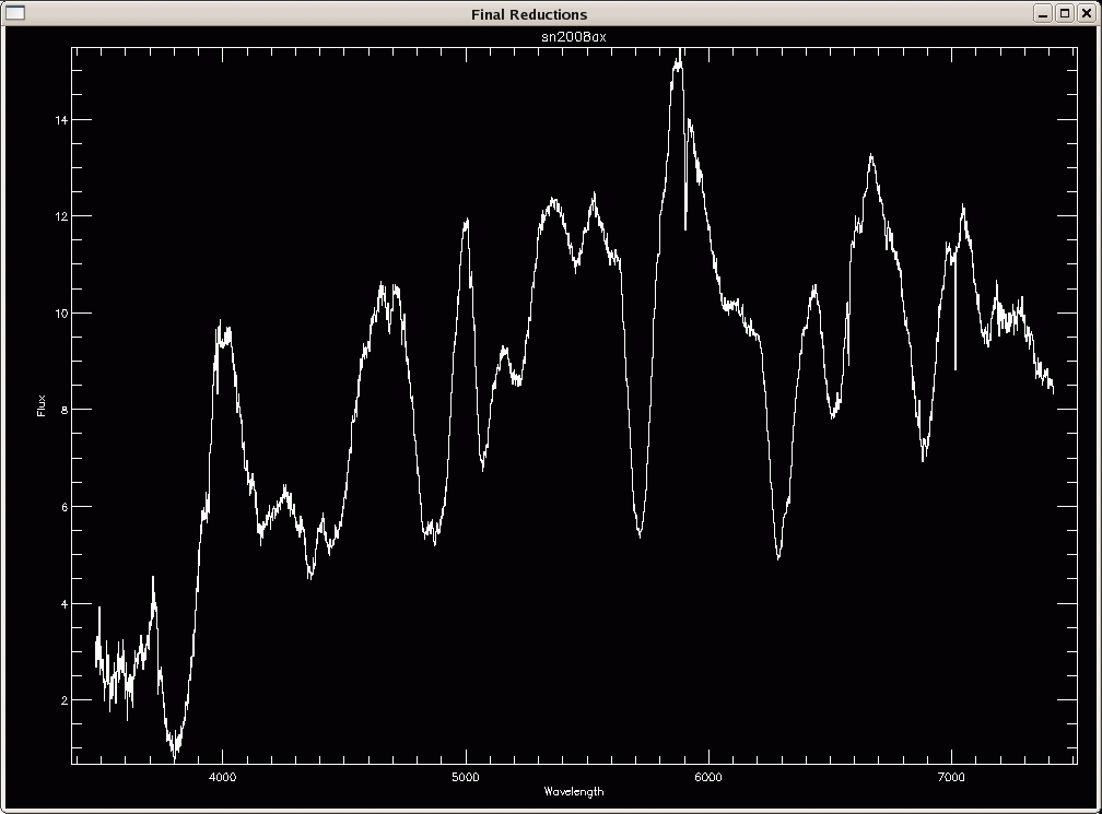
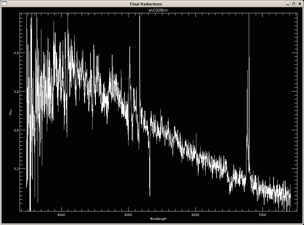
You can see plots of the 7 final spectra below (3 spectra of HD84937, 1 of Feige34, then one of sn2008ax, sn2008bf, and sn2008bm):