Our Milky Way galaxy is a member of the Local Group of galaxies which lies on the outskirts of a large structure of galaxies now called the "Local Supercluster." Although it was first identified on very early sky maps of the distribution of nebulae (e.g. Messier's catalog of nebulae and the New General Catalogue of Dreyer), it was only first recognized as a dynamical entity abouy 50 years ago by Gerard deVaucouleurs after early measurements of the redshifts of its brightest members confirmed that they were generally all in the same volume of space and relatively nearby. DeVaucouleurs (1956) originally called the structure the "Local Supergalaxy," but in 1958 he renamed it the Local Supercluster (LSC). We now know of many structures similar or larger in size, often containing more than one galaxy cluster, and generally called Superclusters.
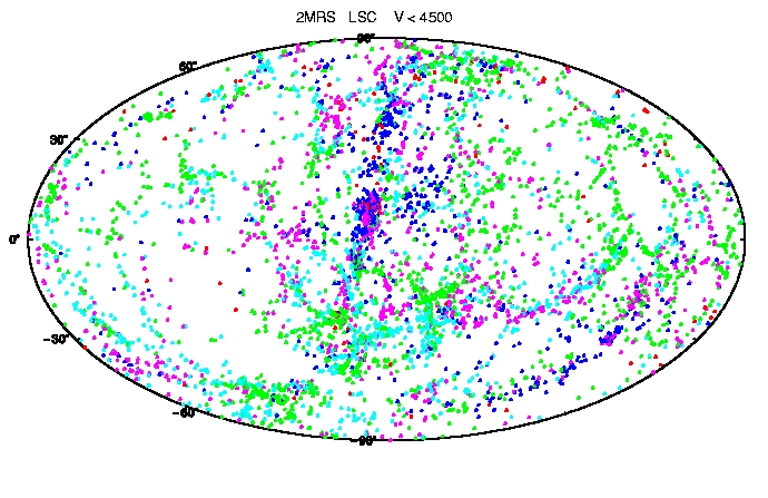
The LSC is roughly centered on the Virgo Cluster, the nearest cluster of galaxies containing several hundred bright galaxies in a volume a few Megaparsecs (roughly 10 million light-years) across. As can be seen by looking at the sky map below, it is a flattened, planar structure with a halo of other groups and clouds of galaxies. The Virgo Cluster itself, subject of another exercise, is at a distance of approximately 16.7 Megaparsecs (55 million light-years) as determined by distance measurements with the Hubble Space telescope.
About 30 years ago, with the discovery of the ubiquitousness of dark matter and the realization that the LSC should have a measurable effect on the Local Group (Peebles 1973; Silk 1973; Gunn)
The purpose of this project is to study the properties of the Local Supercluster with a new and deep all-sky survey of galaxies, the 2MASS Redshift Survey (2MRS). We will measure several global properties of the LSC, including its size and shape. We will examine maps of the distribution of galaxies in the supercluster and the distribution by morphological type.
The data file contains all the galaxies in the 2MRS region around what we think is the center of the LSC. The columns in the ascii file are labeled with their contents. There are several thousand galaxies in this catalog.
This file contains all the galaxies within about 4500 km/s of the Milky Way.
Here is a second file, easier to use, with just the Supergalactic Cartesian Coordinates centered on the Milky Way:
Note that not all the galaxies in this catalog are actually members of the LSC! These galaxies were selected in a sphere around the Milky Way. You will need to transform the object coordinates from our standard spherical coordinates of right ascension, declination and velocity to a Cartesian coordinate system centered on the Virgo Cluster, which is the core of the LSC. For starters, Virgo (given by M87, its biggest galaxy) is at approximately:
Remember that to do the conversion from spherical to Cartesian coordinates you usually have to work with angles in radians, and that the radial coordinate is just the redshift/radial velocity divided by the Hubble Constant (which we will assume is 70 km/s/Mpc) and is thus in Megaparsecs.
Once you have transformed the objects into the x,y,z of the Cartesian system, you can transform again to the center of the Virgo cluster just by adding or subtracting (as appropriate) the x,y,z of Virgo. Then you should "trim" the sample so that you look at (analyse) only those galaxies that are within some distance (perhaps 2000 km/s) of Virgo.
One feature to note in the data is the Virgo cluster itself, at the core of the LSC. A "surface" map of the cluster core reveals a rather complex structure:
If you look at the redshift space distribution (we plot right ascension and the apparent radial velocity), "Virgo Finger," you can see the "Finger of God" effect which is the stretching out of the galaxy positions in "Redshift" space (versus real 3-D "Configuration" space) caused by the rapid motions of the galaxies in the gravitationally collapsed cluster core. Galaxies in the cluster are moving much faster than they would be if they were simply part of the uniform expansion of the Universe --- gravitational collapse and relaxation does that.
I have atttempted to correct the supergalactic x,y,z positions in the data file above for these motions by "collapsing" the redshift space coordinates of the galaxies in the cluster core, defined as being projected within 6 degrees of the center of Virgo, using the approximation formula:
Which should shrink the finger by a factor of six, which is its approximate stretching in Virgo relative to pure Hubble expansion. This of course might make your map look a little funny, but its the best we can do so as not to be dominated by the finger-of-God effect.
P.S. Can you think why the finger in redshift space points back towards the origin (us)? That's why its called the finger-of-God.
What next? The first thing to think about is the definition of the plane of the local supercluster. There is a well known and used definition that dates back to the early days of large galaxy catalogs and that was created/defined by Gerard deVaucouleurs and his collaborators. (See "The Second Reference Catalogue of Bright Galaxies" by deVaucouleurs, devaucouleurs & Corwin.)
A very useful thing to do is to plot the data in various ways. One might be to transform the coordinates to the supergalactic system of dV et al. and plot our catalog in that system. I will look for a way to simply transform our catalog into those coordinates, much the way we transformed RA & Dec to Galactic L and B. But you should think about coordinate rotations. Also remember that we see more of the near side of the LSC than the far side.
What are the questions we want to answer and how can we do that?
A hint on size, we often describe the "sizes" of fuzzy things by contours, either relative to the central brightness or to some mean level. In the case of the galaxy distribution, "overdensity contours" is a popular choice. You essentialy need to calculate the mean density of the sample volume, probably best done with a volume limited sample, and then at each place in the survey, compute the density relative to that mean. Look at the shape of the volume contained by places with densities greater than, say, 2 times the mean or perhaps 1.5 times the mean or something like that.
Another, harder description of "size" is to fit a function to the shape of the density distribution and use a parameter of the fit to define size (e.g. full width half maximum, or the volume that matches the shape of the distribution and that contains half the total luminosity, or something like that.
Some simple plots showing the structures in supergalactic cartesian coordinates are here:
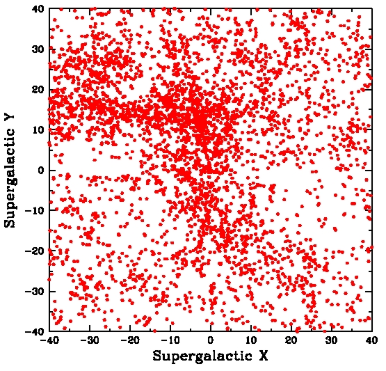
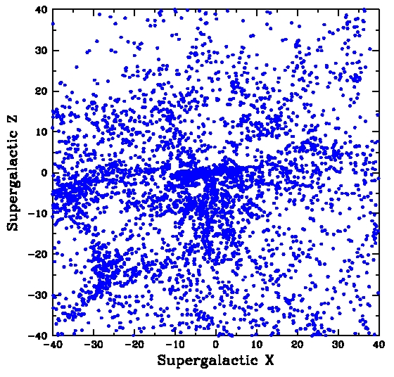
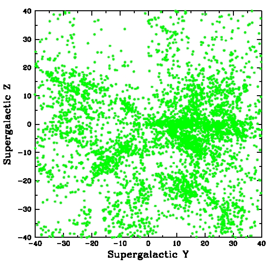
Note that these plots are, like our original data set, centered on the Milky Way. These plots were made using a plotting program/system called Supermongo. An example program is plane.sm . This will run on any of the CfA unix/linux systems provided all the data files are linked correctly and the proper software links are created in your login command file.
The next issue to think about is the fact that our sample is an "apparent magnitude" limited sample. That means we can see pretty much every galaxy nearby but only the most luminous ones at the edge of the sample. The absolute magnitude of a galaxy in the survey is
Where m is its apparent magnitude and D is the distance in Megaparsecs given by its velocity divided by the Hubble Constant --- for us D=v/(70 km/s/Mpc) and is tabulated in the data file. The limiting absolute magnitude for the sample selected for you is thus
However, when you recenter on Virgo and cut again at, say, 2000 km/s around that center, the limiting mag gets a little fainter (we're not looking out quite so far) and becomes something like
That's because we're not in the end looking all the way to 4500 km/s but only 1100 + 2000 km/s. Note that 11.25 is the magnitude limit of our survey (see above).
Thus you can construct a magnitude limited sample by calculating the absolute magnitudes of the galaxies in the survey using the equation above and then creating a new sample, centered on Virgo, but cut to be brighter (more negative) than -22.0. That will be a sample smaller than the one you ended up with after the coordinate shift and radial cut, but it will uniformly sample the volume.
Now that you've transformed the coordinates to the center of Virgo and created a volme limited sample, remap the LSC and see if you can determine size, shape, radial density profile, etc. Remember that if you create "rings" around Virgo to do the density vs r, density will be measured in projection, i.e. as the number of galaxies per Megaparsec squared since we've integrated in the z direction. Good luck!
For those of you who want to delve more deeply into this problem, the last look at the parameters of the LSC was based on an optical survey (The Optical Redshift Survey or the "ORS") and was written up 7 years ago. ORS.LSC Paper That might give you some ideas as to how to measure the orientation and the size and shape of the LSC (hint, think moment of inertia).
References
Copyright John P. Huchra <huchra@cfa.harvard.edu> 2007