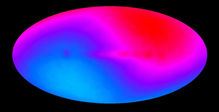
In the mid-1970's, astronomers studying the Cosmic Microwave Background radiation to study the large scale homogeneity of the Universe discovered a startling dipole pattern on the sky. Indeed more modern observations with the COBE (Cosmic Background Explorer) satellite have shown this to be essentially a perfect dipole. The amplitude of the dipole is only 3.358 +/- 0.001 milli Kelvins in the direction (l = 264.31 +/-0.16, b = +48.05 +/-0.09, Galactic coordinates, or RA = 11.199 h , Dec = -7.22, celestial coordinates). The dipole was almost immediately interpreted as a motion of the Milky Way or the whole Local Group. In raw form, since the observation is made from the solar system, its amplitude is only about 369.0 +/- 2.5 km/s and is in a direction almost opposite the rotation direction of the Sun around the center of the MW. After correction to the reference frame (barycenter) of the Local Group of galaxies, however, the velocity amplitude rises to 627 +/-22 km/s towards (l = 276 +/-3, b= +30 +/-2) where the increase in the uncertainty is due to the uncertainty in the coordinate transformation (c.f. Lineweaver 1996).
Even before the discovery of this dipole motion, astronomers had been "sniffing" around the idea that the expansion of the Universe might not be uniform, especially on small scales. For example, we know that the Local Group of galaxies is bound and therefore the galaxies in it are not participating in the global expansion at least relative to each other. We also know that galaxies in the cores of rich clusters of galaxies are bound to those much more massive objects and are in orbit around their centers with "peculiar velocities" that are substantial, thousands of km/s, such that in the nearest rich cluster, Virgo, the gravitationally induced velocity can dwarf the "Hubble" velocity (the velocity due to the expansion of the Universe). In the early 1950's, Vera Rubin (1951) first attempted to measure peculiar velocities in the nearby Universe, and in the mid-1950's Gerard deVaucouleurs (1956, 1958) hypothesized that the Milky Way should actually be falling into (i.e. expanding away from more slowly) the Local Supercluster (c.f. the seminar projects on the Virgo Cluster and on the Local Supercluster).
The fundamental idea here is that the non-cosmological motion of the Local Group would be caused by some large mass concentration pulling us towards it. In other words, Gauss's theorem says that if matter in the Universe were truly uniformly distributed there would be no net force on any galaxy, but since we know that the Universe is lumpy, galaxies will be accelerated by large masses such as othr galaxies, galaxy groups and galaxy clusters that are near them. Since the pull of gravity decreases as the square of the separation, nearby masses have a much greater effect than distant masses. Also, we still do think that on very large scales, in the words of Edwin Hubble, "the Universe is sensibly uniform."
Given that, the first place astronomers looked for the cause of our motion w.r.t. the CMB was the Local Supercluster following deVaucouleurs (c.f. Schechter 1980; Davis et al. 1980; Aaronson et al. 1982). The Local Supercluster dominates the galaxy distribution inside a distance of a few thousand km/s (40-50 Megaparsecs or 120-150 million light years). We found a definite "flow" into the LSC, the Local Group is expanding away from Virgo about 250 km/s slower than it would be if we were freely participating in the Hubble Flow, but that 250 km/s motion is much less than the ~630 km/s and not quite in the right direction.
Since Virgo and the Local Supercluster can't do it, astronomers looked for bigger things further away.
The purpose of this project is to study the properties of the Great Attractor (GA) with a new and deep all-sky survey of galaxies, the 2MASS Redshift Survey (2MRS). We will measure several global properties of the GA, including its size and shape. We will examine maps of the distribution of galaxies in this supercluster and the distribution by morphological type.
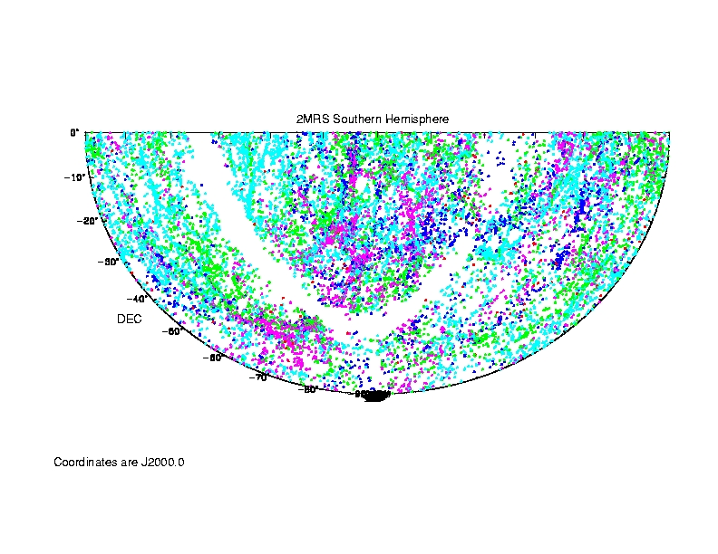
The data file contains all the galaxies in the southern celestial hemisphere and includes what we think is the center of the Great Attractor. The columns in the ascii file are labeled with their contents. There are about 38,800 galaxies in this catalog.
This file contains all the galaxies within about 10000 km/s of the Milky Way, in the southern celestial hemisphere and brighter than a limiting apparent K-band magnitude of 12.5.
Here is a second file, easier to use, with just the Supergalactic Cartesian Coordinates centered on the Milky Way:
Note that not all the galaxies in this catalog are actually members of the GA! These galaxies were selected from a survey centered on (by definition!) the Milky Way.
You will need to transform the object coordinates from our standard spherical coordinates of right ascension, declination and velocity to a Cartesian coordinate system approximately centered on the GA region. For starters, we think that the GA may be roughly centered on the galaxy cluster Abell 3627, which is is at approximately:
Remember that to do the conversion from spherical to Cartesian coordinates you usually have to work with angles in radians, and that the radial coordinate is just the redshift/radial velocity divided by the Hubble Constant (which we will assume is 70 km/s/Mpc) and is thus in Megaparsecs.
Once you have transformed the objects into the x,y,z of the Cartesian system, you can transform again to the center of the GA just by adding or subtracting (as appropriate) the x,y,z of the GA. Then you should "trim" the sample so that you look at (analyse) only those galaxies that are within some distance (perhaps 3 to 4 thousand km/s) of the GA.
If you look at the redshift space distribution (we plot right ascension and the apparent radial velocity for the sample above), you can see the "Finger of God" effect which is the stretching out of the galaxy positions in "Redshift" space (versus real 3-D "Configuration" space) caused by the rapid motions of the galaxies in the gravitationally collapsed cluster core. Galaxies in the cluster are moving much faster than they would be if they were simply part of the uniform expansion of the Universe --- gravitational collapse and relaxation does that.
P.S. Can you think why the finger in redshift space points back towards the origin (us)? That's why its called the finger-of-God.
What next?
A very useful thing to do is to plot the data in various ways. One might be to transform the coordinates to the supergalactic system of dV et al. and plot our catalog in that system. Look for a way to simply transform our catalog into those coordinates, much the way we transformed RA & Dec to Galactic L and B. But you should think about coordinate rotations. Also remember that we see more of the near side of the GA than the far side.
What are some of the questions we want to answer and how can we do that?
A hint on size, we often describe the "sizes" of fuzzy things by contours, either relative to the central brightness or to some mean level. In the case of the galaxy distribution, "overdensity contours" is a popular choice. You essentialy need to calculate the mean density of the sample volume, probably best done with a volume limited sample, and then at each place in the survey, compute the density relative to that mean. Look at the shape of the volume contained by places with densities greater than, say, 2 times the mean or perhaps 1.5 times the mean or something like that.
Another, harder description of "size" is to fit a function to the shape of the density distribution and use a parameter of the fit to define size (e.g. full width half maximum, or the volume that matches the shape of the distribution and that contains half the total luminosity, or something like that.
The next issue to think about is the fact that our sample is an "apparent magnitude" limited sample. That means we can see pretty much every galaxy nearby but only the most luminous ones at the edge of the sample. The absolute magnitude of a galaxy in the survey is
Where m is its apparent magnitude and D is the distance in Megaparsecs given by its velocity divided by the Hubble Constant --- for us D=v/(70 km/s/Mpc) and is tabulated in the data file. The limiting absolute magnitude for the sample selected for you is thus
However, when you recenter on the GA region or about 4000 km/s and cut again at, say, 3000 km/s around that center, the limiting mag gets a little fainter (we're not looking out quite so far) and becomes something like
That's because we're not in the end looking all the way to 10,000 km/s but only 4000 + 3000 km/s. Note that 12.5 is the magnitude limit of our survey (see above).
Thus you can construct a magnitude limited sample by calculating the absolute magnitudes of the galaxies in the survey using the equation above and then creating a new sample, centered on the GA, but cut to be brighter (more negative) than -22.0. That will be a sample smaller than the one you ended up with after the coordinate shift and radial cut, but it will uniformly sample the volume.
Now that you've transformed the coordinates to the center of the GA and created a volme limited sample, remap the LSC and see if you can determine size, shape, radial density profile, etc. Remember that if you create "rings" around the GA to do the density vs r, density will be measured in projection, i.e. as the number of galaxies per Megaparsec squared since we've integrated in the z direction. Good luck!
References
Copyright John P. Huchra <huchra@cfa.harvard.edu> 2007