Data reduction for MEarth follows the general philosophy described in Irwin & Lewis (2001) and Irwin et al. (2007) (see also Irwin 1996 for a more general overview of CCD reductions for wide-field imaging). However, there are a number of instrument-specific problems detailed below that require additional processing steps or modifications to the standard procedure. These are listed in roughly the order they are done by the software.
Although this is not a modification to the normal procedure, it is worth stating that the MEarth detectors, like nearly all CCD systems, show some non-linearity. Non-linearity corrections were derived from sets of "dome" flats taken using daylight to illuminate the roof on a clear day, with careful attention given to monitoring the illumination level and correcting for variations.
Dark current is not negligible in MEarth data: although the overall level is quite low, there are quite a lot of hot pixels, particularly at the -15C operating temperatures used until the detector housings were upgraded during the 2011 summer monsoon. Experience shows the number of hot pixels is a function of device temperature. Moreover, the hot pixels do not seem to be completely stable from night to night.
After the upgrade, the persistent image of the pre-flash lamp pattern is visible in the dark frames.
Dark frames are taken every night (at the end of the night). This uses a fixed exposure time (it would be prohibitively expensive to do all exposure times used for targets). This means hot pixels are imperfectly corrected because they seem to be somewhat non-linear with exposure time.
Dark frames before 2010-02-26 were affected by the persistent image of the dawn twilight flats (where taken) due to starting darks too soon after closedown. The persistent image would gradually decay away during the sequence of darks, but was still present in the average master dark used to correct the data. A delay to allow the persistent image to decay away before starting darks was added on 2010-02-26.
The use of a leaf shutter necessitates a correction for the non-uniform exposure across the field-of-view due to shutter travel time. This is a ~5% effect on a 1 second exposure. The correction seems to be fairly stable over few month timescales, and was derived from sets of twilight flats (to measure the pattern) and a dedicated sequence of short-exposure dome flats using bright illumination (to measure the travel time / normalization). The correction is applied in two parts: the non-uniform pattern at the image level, normalizing to the median of the shutter map; and the travel time / normalization of this map itself is applied to the exposure time stored in the headers. The correction is imperfect due to the illumination change over twilight and evolution of the travel time over approx. 1 year timescales, but should be sufficient for the majority of MEarth photometry. Note that the number of shutter blades increased from 5 to 6 when the housings were upgraded at the 2011 summer monsoon, but the travel time is still similar.
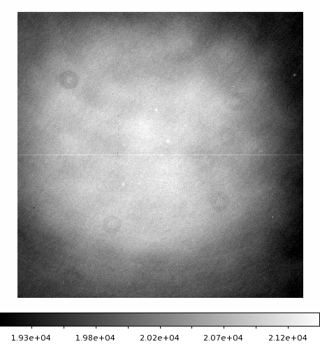
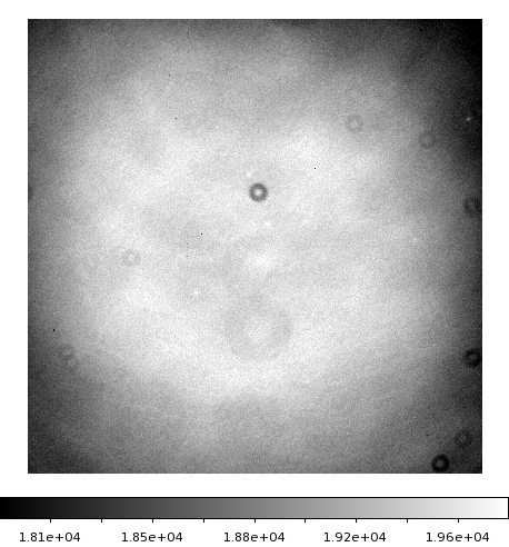
Experience shows that the standard (simple) method of taking twilight flats produces a result that is not uniform to better than the several percent level. Instead, as of 2008-10-29, twilight flat fields are taken on alternating sides of the meridian to mitigate most large-scale illumination effects (the detector rotates by 180 degrees relative to the sky upon crossing the meridian, so gradients tend to average out). Before the summer 2011 detector upgrade, the center was affected by a severe case of "sky concentration" / "scattered light" to the tune of about 10% (in 2008-2010) or 15% (in 2010-2011) of the sky level at peak. Some experimentation led to the current ad-hoc working solution, which is to divide out a Gaussian fit to just the center portions, to remove the "scattered light", followed by dividing out all the large-scale illumination components using a 2-D median filter (except these steps were reversed in 2008-2010 processing). This leaves essentially only (a) dust doughnuts, and (b) the pixel to pixel response variations. The "correct" illumination part was then derived photometrically and multiplied in to the final flat field used to process the images. This seems to be quite stable and was done by dithering a dense star-field around the detector, making an image of the photometric residuals using a Kernel Density Estimation type of procedure with a Gaussian kernel of roughly the image FWHM, and smoothing the result to produce the final map. The final flat-fielding appears to be good to about a percent, but there is clear evidence for residual errors in the form of "meridian offsets" in the light curves. The 2008-2010 illumination map was rather inferior quality compared to the 2010-2011 one since a lot of improvements were made to the methodology. The 2008-2010 map was derived from the same observations taken of target fields during loss of pointing refinement as the fringe maps (see below) rather than dedicated fields with a very high stellar density, so was lacking in terms of sampling.
After the 2011 summer monsoon, the scattered light has been substantially reduced thanks to improvements made to the baffling close to Cassegrain focus, and upgraded anti-reflection coatings on the CCD window. The Gaussian fitting step is no longer needed. Otherwise, the flat fielding procedure is the same, since there is still some scattered light. Also note that the scattered light pattern is different in the South compared to the North due to differences in the telescope baffle design.
The raw data from MEarth-North show substantial fringing due to the combination of a very red bandpass and thinned, back-illuminated detectors. However, before the detector upgrade the devices also showed a strong persistence effect (see below), which made it very difficult to generate a usable dark sky flat ("fringe map") with which to correct this effect. The fringe maps were derived from observations taken in 2008 December during a week when the pointing refinement was not working, so the target fields drifted all over the detector, but these were getting outdated by 2011, and the fringe correction was noticeably inferior during 2010-2011 after the filter had been changed. The situation was substantially improved in 2011-2012 and later seasons, where fringe frames were much easier to derive and therefore could be updated more often.
Defringing is done by first removing large-scale structure in the image (the smoothing box is 256 pixels) to remove the "glow" (see below). The fringe map is then compared to this and an "optimal" scale factor determined. The scaling is first guessed using the ratio of sky levels and then refined adaptively, this is necessary to track variations in the (predominantly OH) emission that causes the fringes. Finally, the scaled fringe pattern is subtracted from the original image. The fringe pattern itself is found to be very stable over time, and appears to essentially be an intrinsic property of the device.
The Southern detectors have an anti-etaloning NIR coating and do not show substantial fringing, so it is not corrected.
The "blind" pointing of our mounts (after application of a standard pointing model) is not sufficient to achieve the approx. few pixel rms accuracy required to mitigate the effect of flat-fielding errors in the photometry. The observing system uses short, binned exposures to refine the pointing (these are not saved) before taking the main science image. Sometimes, this can fail, and the science images are still taken regardless. A "blind" pointing solution based on the astrometry.net project was added to allow frames where the pointing was very far off to be solved properly. Starting with DR4, final astrometric calibration is now done using the UCAC4 catalogue (previous releases used 2MASS), and typically achieves RMS residuals below 0.1 arcsec in low wind (worse for long exposures in windy conditions due to wind shake).
It should be noted that occasional losses of pointing refinement have been experienced due to failure of the Windows COM (common object model) communication between the telescope control software and the CCD control software after the system has been up for several weeks. It is not known why this happens, but it requires a reboot to fix. Procedures for ensuring this cannot affect science data by scheduling regular reboots and reporting errors to the operator in a more visible fashion have prevented the problem occurring in recent data, but occasional half-nights have been affected in earlier data, and there was one several night long stretch in 2008 December when the usual operator was on vacation (which has been used for calibration purposes as detailed above).
These are useful for removing bad data before attempting differential photometry. Magnitude zero-points are computed for each individual observation, based on standard stars within the field from APASS. This is done as part of real-time and offline (final) analysis.
The observing system tries to get one image of each of a set of 8 equatorial standard star fields containing multiple standard stars from Landolt (1992) every night. These are used to compute photometric zero-points in the usual way. Note that these solutions presently do not solve for the atmospheric extinction, so the accuracy of this procedure is limited by any variations. For any serious purposes it is currently necessary to manually derive the extinction coefficient for the night in question. Note that the zero-points are computed regardless of weather, but the results will not be accurate in non-photometric conditions!
This is essentially identical to the Monitor methodology (Irwin et al. 2007), with a few minor exceptions. Because our stars have high proper motions, it is necessary to have the apertures follow them. This starts off with a guess based on the catalogue proper motion, and then refined by allowing the centroids to move to account for any errors before doing the final photometry.
For the light curves, the most major change of relevance was the addition of a per-star "meridian flip offset", solved along with the per-star magnitudes so the weights (derived empirically from the RMS scatter in the light curves) used to compute frame zero-points are not artificially squashed at the bright end by including meridian offsets in the RMS estimates. Frames are normalized using a simple non-spatially varying zero-point offset, rather than the polynomial fit described in the paper, to avoid overfitting when there are very few comparison stars. The per-star magnitudes' zero-point is tied down by forcing the median difference of these compared to the reference ("master") frame to be zero. If the master frame was taken in photometric conditions and was correctly photometrically calibrated, the magnitudes in the light curves should also be properly calibrated in an absolute sense. Due to the uncertainty about whether this calibration is correct, it is currently removed in the released light curves, which are purely differential measurements.
Aperture sizes: aperture photometry is computed in a series of concentric apertures, at factors of two in area, starting from a base aperture radius r of 5 pixels in the 2008-2010 Northern data, 4 pixels in the 2010-2011 and all later Northern data, and 3 pixels in the Southern data. The light curves use apertures of r, sqrt(2)*r, 2*r, and for the 2008-2010 Northern data and all Southern data, 2*sqrt(2)*r. The one showing the lowest RMS scatter in the final light curve is adopted (due to variability, this scheme is not optimal, and may be revised in the future). The sky annulus is 6*r to 8*r, and the sky level is computed from the pixels in the sky annulus using an iterative, clipped median.
During the 2008-2009 season, the telescopes were operated intentionally out of focus, adjusted to achieve FWHM of approx. 5 pixels (where a normal in-focus FWHM is approx. 2.5 pixels) in order to be able to collect more photons per exposure before saturation. It was found to be very difficult to maintain a stable defocus, and the FWHM varied substantially with changes in ambient temperature. Stabilizing this was hindered by failure of the focus drive electronics on many of the telescopes. As a result, these data have rather unique systematics and many other related problems.
For the 2009-2010 season, the decision was made to operate in focus, and to take multiple exposures per visit to a given target where required to achieve adequate signal to noise. Continued failures of the telescope focus drive electronics throughout this season severely hampered attempts to keep the telescopes in focus and stable, and these problems were not fully rectified until some replacement electronics were procured for telescopes 2 and 6 during the 2010-2011 season, although the situation was substantially improved already by 2010 startup.
During the 2008-2009 season, the temperature setpoint was -20C, which proved to be too optimistic, and became difficult to maintain during the summer. The setpoint was changed to -15C for the 2009-2010 season. During the 2010-2011 season, problems were experienced with the cooler on telescope 2, so the setpoint for this telescope was changed to -10C at the start of the season. The setpoint on telescope 5 was adjusted to -10C on 2010 December 10 due to concerns about condensation in the CCD chamber. The device operating temperature during these seasons was a particular concern due to persistence (see below). Since 2011 October, the operating temperature has been -30C, and has remained stable.
Numerous problems were experienced with condensation in the CCD chambers leading to formation of ice crystals on the CCD at the start of the 2009-2010 and 2010-2011 seasons. After the detector housing upgrade in 2011-2012, all of the shutter driver transistors eventually failed, and were dealt with as needed during the season. There have also been occasional shutter failures and readout electronics failures. All of these incidents required removing the detector from the telescope and shipping it for repair, and these were occasionally returned with the electronics adjusted, meaning the gain was altered and it was necessary to re-do all of the calibrations. Additionally, the gain was intentionally altered to make better use of the full-well capacity of the CCDs during the 2011 Summer detector housing upgrade.
A separate log has been maintained showing the dates of all changes for each telescope, and the data files contain an "instrument version number" that increments by one every time a detector was taken off and put back on. The light curves are split every time there was such a change, and the software solves for separate per-star magnitudes and meridian offsets on either side of the change due to the expected discontinuity in flat-fielding error. The influence of these changes on the photometry is unfortunately exacerbated by a lack of precision and repeatability in the adapter used to align the detector axes with the cardinal axes (and telescope optics), which is approx. 0.5 degree at best.
The telescopes are extremely prone to wind shake as used in the present enclosure (which has minimal protection from wind). This results in distorted PSFs in moderate wind, becoming severely distorted in high winds approaching the close-down limit for the enclosure. Due to the design of the building, this affects each telescope differently, and also depends on wind direction. At Mt Hopkins, winds from the East, Northeast and occasionally Northwest can also result in extremely poor seeing. This is noticeable in MEarth images even though the intrinsic PSF FWHM is approx. 2 arcsec, which normally renders them relatively insensitive to seeing variations, and can often be distinguished from wind shake by lower winds and circular PSFs.
Images tend to show visible PSF distortions in winds exceeding 15 km/h, and it is likely there are astrometric distortions at even lower wind speeds. The effect on image quality also depends on the nature of the wind with gusty conditions tending to produce a mixture of undistorted and highly distorted frames. Because aperture photometry is used with large apertures, the light curves are remarkably insensitive to these problems, but there is a noticeable trend of large scatter (often caused by a poor zero-point solution) in high wind. These images can usually be detected by examining the FWHM and ellipticity parameters, although the most distorted frames are known to fool the source classification procedure, which can result in no estimates of FWHM or ellipticity being made because it didn't think there were any stellar sources on the frame, which appears in the output as FWHM = -1.0. It should also be noted that the achieved pointing error is degraded in high wind.
The mounts natively (before correction) show a small amount of periodic error, which can cause image elongation in the y (RA) direction for long exposures. The worm period is 2.5 minutes, so these effects are most pronounced for exposures longer than 30 seconds or so. However, the effects can also show up in high-cadence continuous sequences of exposures taken for transit followup or similar, where it leads to excess scatter in the y coordinate time-series. It is possible for the periodic error to interact badly with the pointing stabilization software loop used during these observations, and this can increase the size of the error since the feedback attempting to fix the worm error occurs out of phase with the error itself.
Periodic error correction has been used since 2010 January to address this problem. The periodic error curves are based on measurements of the error averaged over approx. 20-25 worm cycles, using a dedicated set of very high-cadence short exposures on a bright, equatorial star taken during low wind. However, it is found that the solutions need to be updated quite frequently (every few months) as there is some drift in the worm error over time. This has occasionally lagged due to the special conditions (extremely low wind) needed to obtain a good calibration or because it was not noticed quickly. The periodic error can change dramatically when the mounts are re-lubricated, so the calibration is always re-run at these times (annual, at startup after the monsoon).
The difficulty here is really that it is not possible to tell the mount decided to flip until it is too late, because the only way to know is by solving astrometry on an image. The target acquisition software attempts to detect flips between the first and second acquisition exposures and starts over if one is detected. But flips after the second acquisition exposure show up in the science image, because they evade detection until it is too late (the telescope has already slewed to the next target by the time the science image can be analysed). Worse still, the pointing error vector is typically reversed on flip, so the resulting error is roughly double the native mount pointing error because the correction ended up applied backwards. Thankfully, this doesn't happen very often.
Flips during continuous observations (high cadence followup) are more of a problem. Once a flip is detected, the situation is treated as a reacquisition, but this was buggy for many years due to lack of use and consequently, limited testing. The pointing stabilization loop uses a proportional-integral-derivative filter to prevent oscillation (the additional complexity over an auto-guider, which usually only does the proportional part, is needed because the images being used are the science images, so the feedback is very slow, and the gradual "drift in" that results from a pure proportional feedback turned down low enough to stop oscillating was not adequate when tested). The impulse response of such a loop is ideally similar to that of a critically damped harmonic oscillator, but tuning errors are inevitably present in a real implementation, particularly as the loop has not been individually adjusted for each mount. This is clearly seen in the pixel coordinate time-series after a meridian flip during a continuous observation and can temporarily disrupt the photometry until the loop settles to its new equilibrium.
Some continuous observations have flipped three times when they arrived at the meridian, because the requested pointing after the first flip and acquisition exposure with the new pointing error correction vector applied happened to be on the other side of the meridian again (temporarily!).
The use of commercial data acquisition software and the Windows operating system causes difficulty with achieving accurate time stamps. Consequently, they are only good to a few seconds at best, and until 2014 September were only written out to the FITS headers to one second precision.
DR1 presented the light curve time stamps in Heliocentric Julian Date (HJD) in the UTC time-system, correcting only for the motion of the Geocenter relative to the Sun using the Stumpff (1980) routine to compute the appropriate state vector, and did not allow for source proper motion between the master frame and the frame being reduced. This has now been changed (for DR2 and all subsequent releases until further notice) to use Barycentric Julian Date (BJD) in the TDB time-system. The treatment used to compute this quantity (see here) includes many more corrections, and is based on the JPL DE430 solar system ephemeris. It should be at least three orders of magnitude more accurate than the input UTC time stamps from the data acquisition system, given the astrometric quantities stated in the file headers.
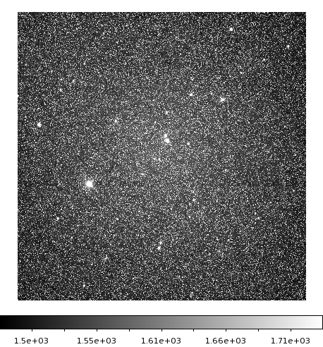
All taken from tel05 on 2011-02-21 and 2011-10-22 (nights of), where the former date was before the housing change, and the latter after the housing change. In cases where the calibration has changed significantly after the housing upgrade, both are shown (before the change, then after the change; most browsers should display them side-by-side with before on the left, if the window is wide enough), otherwise only the one from before the housing change. Only the bias, dark, and high frequency component of flat are derived per night, all other calibrations were those considered current when that night was reduced.
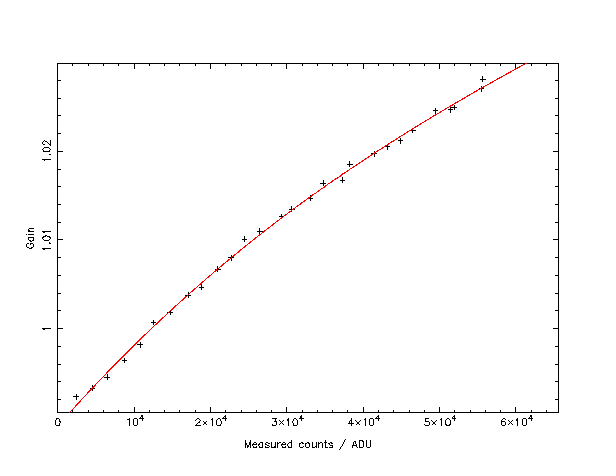
The quantity on the vertical axis in this plot is the ratio of measured sky level to the reference sky level, scaled by the ratio of exposure times. The reference frames were exposed around 13,000 ADU and interleaved between the target frames to track variations in the illumination of the roof. Counts in this diagram are raw, not de-biased, but were corrected for shutter shading. The curve is a simple polynomial:
actual = raw (1 + c_1 * raw + c_2 * raw2 + c_3 * raw3)
This assumes the two (should) agree at 0. It doesn't matter exactly where things are normalized, as this is removed by the photometric calibration, and is factored into the gain measurement by computing the gain from dome flats that have already had the non-linearity correction applied.
Please note that saturation on the CCD (the full-well capacity) was below 65535 counts on many of the detectors before the housing upgrade, and all of them afterwards.
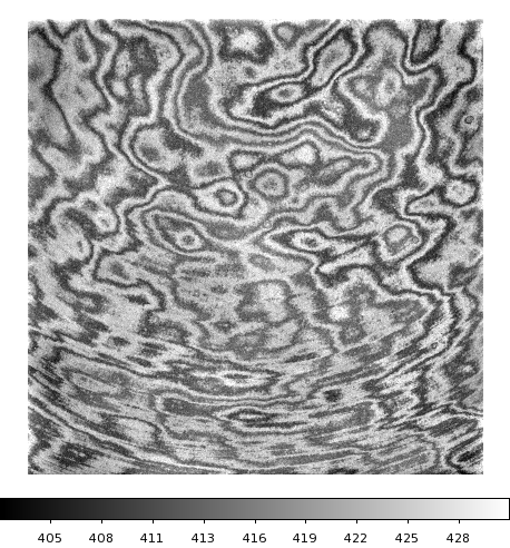
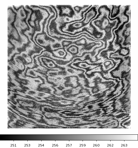
(derived from twilight flat sequences; low-pass filtered to remove noise; note change in number of shutter blades post-upgrade)
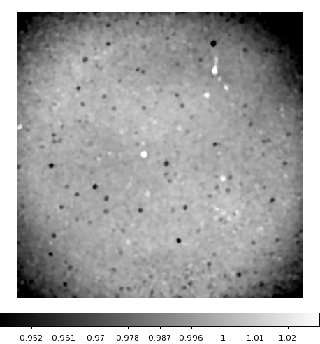
Raw
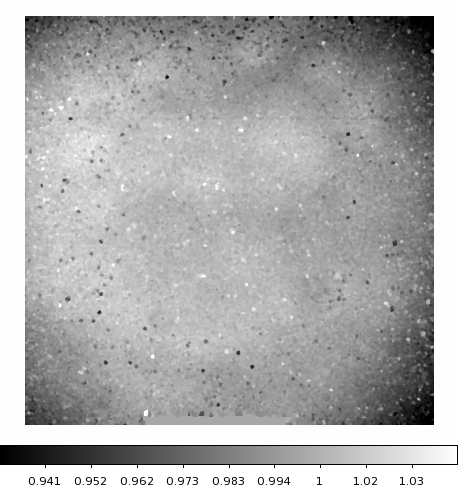
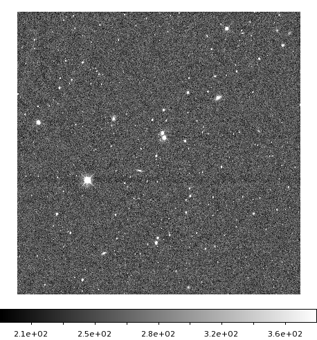
After glow removal
(Elliptical Gaussian fit and subtracted, 2008-2010 and 2010-2011 seasons only)
Low frequency structure removed
(2-D median filter with median box=171, linear box=131)
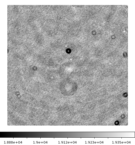
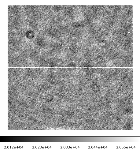
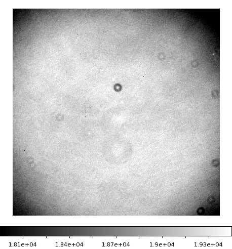
The first of these illustrates a known issue with the glow removal, due to the unfortunately placed dust doughnut near the center of the field.
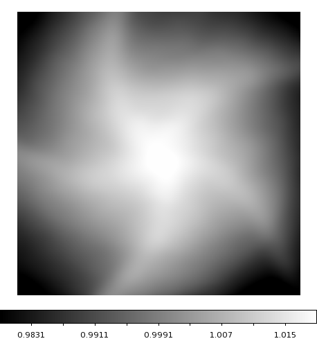
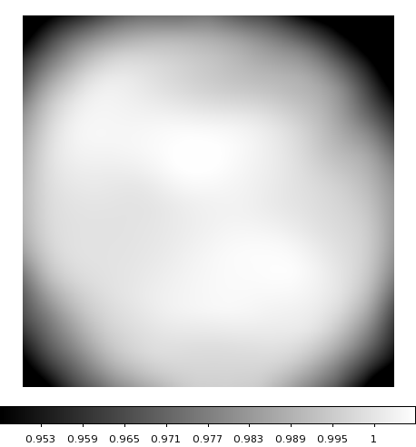
Illumination map (raw)
Or, "photometric flat"; determined by dithering a star-field around the detector, by random offsets, many times, and doing photometry of all the stars. This image contains a Gaussian scaled proportional to the measured flux ratio wherever there was a measurement.
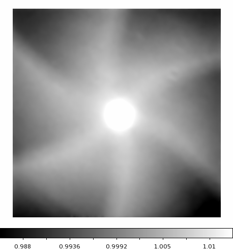
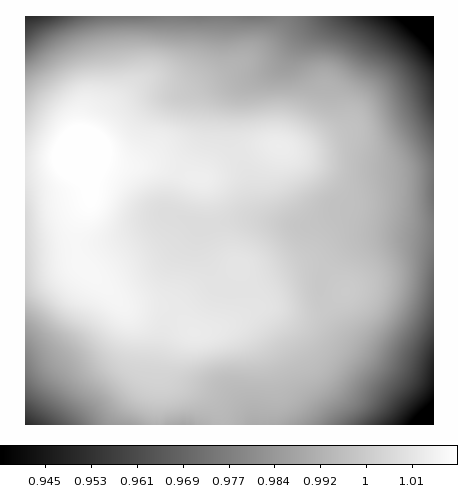
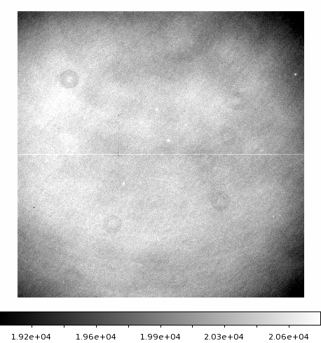
Illumination map (smoothed)
(2-D median filter with median box=301, linear box=211)
Final
Also filtered, low-pass to remove noise, and high-pass to remove scattered light. Most of the change below results from adjustments to the filtering parameters, and not in the device itself.
Masks were derived by hand. They are not shown here because the majority of the features are too small to show up in a binned map. The bad pixel masks are used by the source detection and all later stages in the processing.
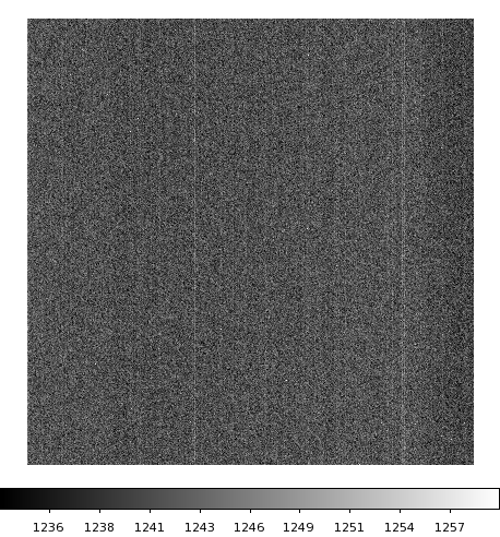
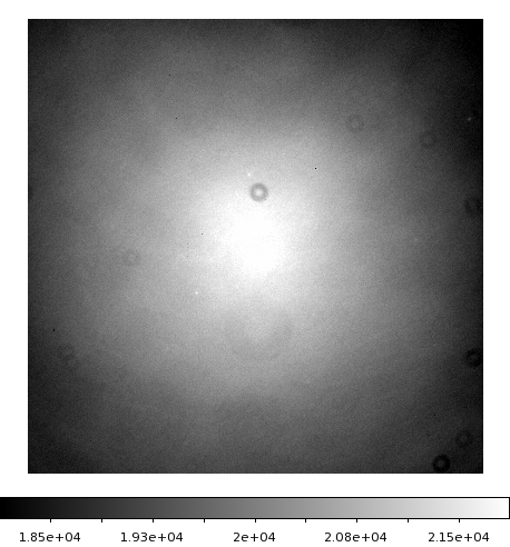
(t05.obj.20110221.00022.fit, before on the left, after on the right)
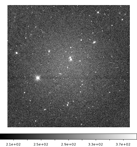
Notice particularly two clearly visible defects that are not fixed by the standard processing. (1) the "glow" in the centre of the field, caused by scattered light. (2) the "pulldown" in rows containing bright stars.
If we had not removed the "glow" from the flat, we would have divided most of it out of the image, so it would look flat, but would not actually be flat (in a photometric sense). The "glow" (scattered light) is thought to be an additive effect, not a multiplicative one (essentially, a fraction of sky is scattered into a Gaussian-like image on-axis).
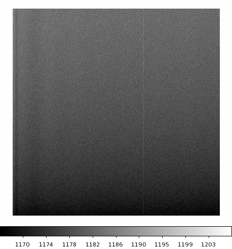
Below is the same image after sky background removal, as used for source detection and photometry (plotted with detected sources overlaid on the right):
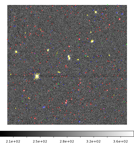
(see Irwin 1985 for details of how this works; sky background following box size was 64 pix)
The source classification has been used to colour the symbols overlaid on the image, and is used to select potential comparison stars. This essentially works by determining the locus of stellar sources in flux vs flux ratios between different sized apertures, and then folds in ellipticities. In this image, red = stellar (PSF-like), blue = non-stellar (i.e. galaxies), yellow = blended (or more accurately, sources with overlapping isophotes), and green = junk-like (usually "cosmics" or hot pixels, essentially sources that are too sharp to have been through convolution with the PSF as determined from the stellar images).
No attempt has been made to fix the "pulldown", due to concerns about making the correction robust against real sources in the same lines, given that there is no overscan region to use for a line-by-line overscan subtraction (or similar). The Southern detectors do not seem to show the "pulldown" so this particular issue only affects Northern data.
No corrections are attempted for this effect (it depends on the full illumination history of the pixel, including the field acquisition exposures, which are not saved).
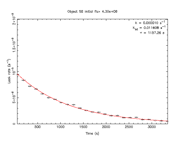
The quantity on the vertical axis of this plot is the fraction of the initial counts (shown at the top) that accumulate in the dark current per second of integration time. This is the integral over a photometric aperture (it was done on stars) so in practice includes a "flux-weighted" range of illumination levels. The model fit assumes the flux decays by a simple exponential law exp(-t/τ). This τ value (20 minutes) is fairly typical of our detectors. The level might seem small, but 43 ADU x 60 seconds (typical exposure) is a quite detectable source above typical sky.
Note that both the normalization, and timescale, in this plot are thought to be temperature dependent, in the sense that with decreasing device temperature, the normalization decreases, and the timescale increases.
During the 2011 summer monsoon, the detector housings were upgraded to Apogee's "high cooling" D09 housing, which allowed a lower operating temperature (-30C) and also added a preflash feature using IR LEDs, which is used on all data taken since the upgrade. The combination of these has rendered persistence to be practically no longer a concern for all data taken 2011 October onwards (it would not be true to say it removed persistence, of course, because we have really done the opposite - the preflash floods the detector with a big persistent image, but in doing so makes it stable; the persistent image then behaves simply as if it was an elevated dark current and is removed by dark frame subtraction).
Our standard astrometric analysis now uses the UCAC4 catalogue, and thus is tied to ICRS. Previous releases used 2MASS.
There is relatively little of note for the calibration itself. There appears to be almost no radial distortion in the data, as expected given the optical system. The derived values vary from telescope to telescope, but they are all at negligible levels and do not need to be corrected. A standard Gnomonic (RA---TAN, DEC--TAN) projection is used.
Substantial contributions and assistance from Mike Irwin, Christopher J. Burke, Philip Nutzman, and the entire MEarth team are gratefully acknowledged.