SMA SWARM Data Calibration with MIR/IDL
WARNING: Parameters used assume data rebinned by a factor of 4. Values for ntrim, preavg, and smoothing should be scaled by any rebin factor.
|
(1) Open MIR/IDL
| |
|
(2) Read the data into MIR
Read in only the 240GHz to ensure there's sufficient memory for processing. It is always advisable to process each receiver separately.
View a summary of the data.
| |
|
(3) Flag pointing data
Pointing data will have an integration time < 6 seconds. It used to be sufficient to select scans that were shorter than this using dat_filter and then flag them.
Since mid 2019, the potential science scan length has been considerably shortened, meaning it is not reliable to blindly flag the pointing scans in newer data based on scan length. Instead a pointing flag has been implemented, and dat_filter can be used like so.
If you are unsure, try flagging by pointing option first. If this does not return any results examine your data to see if any pointings need flagging and what the scan lengths are. Afterwards, you must re-select only the positive weighted (unflagged data). Some scans will have been flagged during the observation (e.g. while the antennas are switching sources) so this will exclude them also.
| |
|
(4) Inspect the data visually
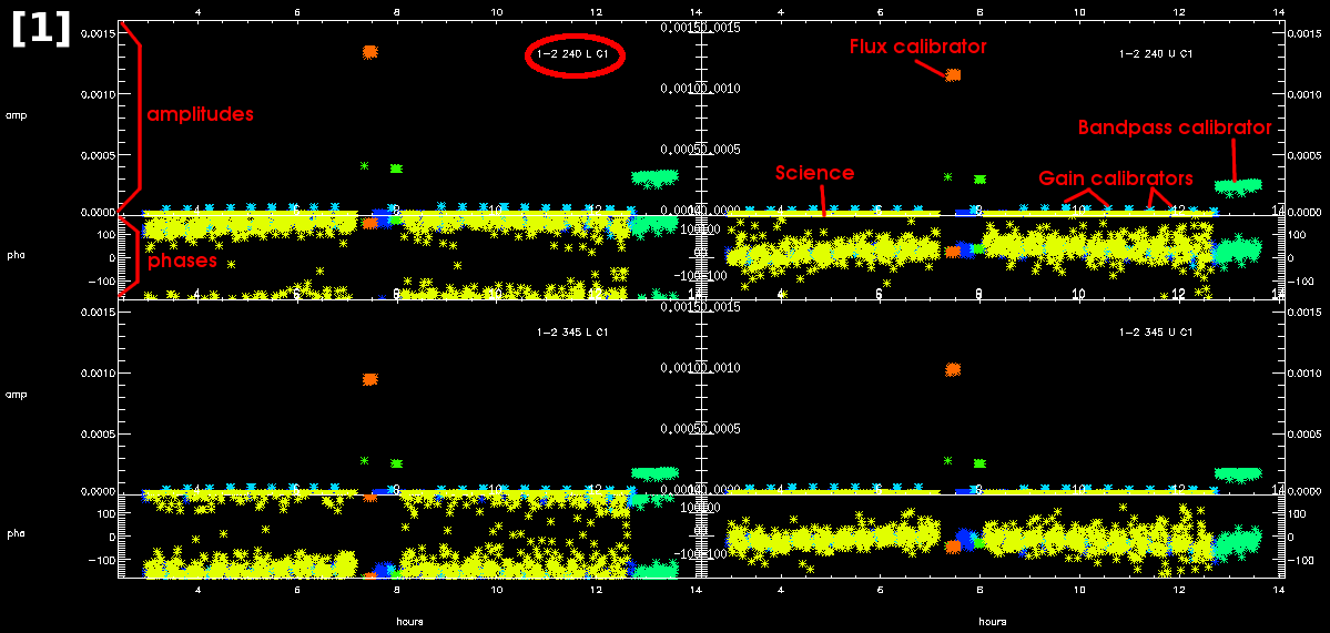
Plot the pseudo-continuum channel [1]. This is an average of the spectral channels across all baselines for each point. Its designation is 'c1'.
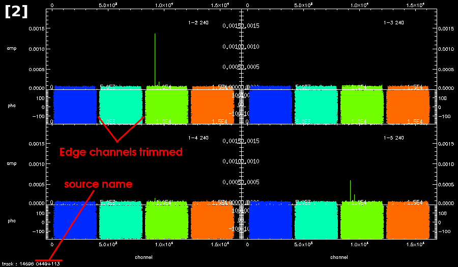
You can also plot the spectral data [2]. Here the noisy edges of the chunks have been trimmed. It is normal to trim 8-10% of the data. For full SWARM resolution of 16384 channels per chunk, 8% is ~1300 channels. As this data has been rechunked by a factor of 4, ntrim is set to 320 (or ~8% of 4096 channels). Note that for x='channel' the units of ntrim are channel number, while for x='fsky' the units are MHz.
The option color='band' makes each chunk a different color. The plots are shown source-by-source so right-click to scroll through them all. You can see any frequency spikes and remove them in the next step. |
|
|
(5) Check for spikes
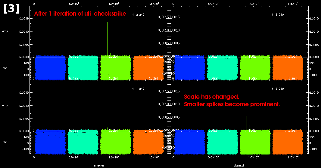
The MIR task, uti_checkspike, will identify and optionally fix spikes in the frequency data. Alternatively, this can be done manually which is more labor intensive but may be faster. This example runs a couple of loops of uti_checkspike, then manually removes a remaining spike. For uti_checkspike a source must be specified. This source will be used as a template to identify the spike positions. As such, choose a source like a gain calibrator quasar, or the bandpass calibrator, which has a flat spectral signature.
The /fix option applies the corrections for each spike identified. When a channel is flagged, it is flagged for all sources. By default the spectra are averaged over all baselines, but the option /baseline finds the spikes in each baseline independently. Be warned the /baseline option takes a long time to complete, and with the very high resolution of SWARM it is often not necessary to worry about losing the occasional channel. Another option is threshold; this is the rms threshold above which a spike is identified. This is 10 by default by can be changed using threshold=X. Checking the spectral plots again show some spikes remaining [3].
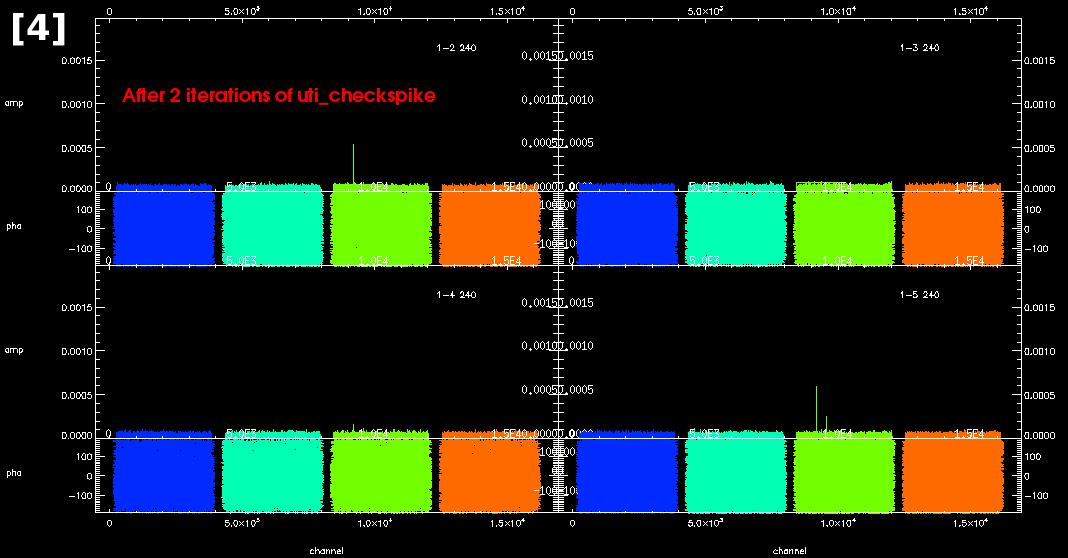
Repeatedly run uti_checkspike so it iterates down [4]. The default threshold over which emission qualifies as a spike is 10-sigma. This can be changed with the option threshold=x.
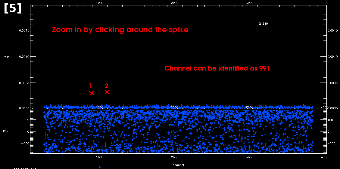
By repeatedly zooming in on the first panel (left-click on the panel, then left-click on ether side of the area to be enlarged), the channel containing the spike can be identified as 991 [5]. Right-click to exit from the enlarged view. Then apply the fix.
By default, uti_chanfix replaces the value of the given channel with an average of the adjacent 3rd channel on each side. You can select which channels will be used to produce the average with the option 'sample'. If a spike is a few channels wide for example, using sample=10 will use the 10th channel on either side for an average. The 'sample' option can also be used with /fix for uti_checkspike. |
|
|
(6) Apply the system temperature correction
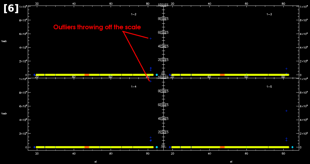
View the system temperature. Check the points and profile for outliers.
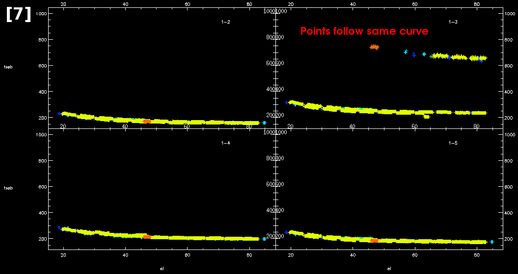
The scaling of the plot is thrown off by some outliers [6]. Here there was a problem recording the Tsys - the data itself are unaffected. Check underlying causes by looking at the observing report to see if any issues were reported. To re-scale the y-axis select data with the range of Tsys to be plotted (here <1000K); then plot that subset [7]. Now points that are offset from the standard curve become visible. Remember to re-select all the data afterwards.
All these points can be fixed using the MIR task uti_tsys_fix. This refits the Tsys for points below 'high=X', and above 'low=Y'. It then replaces any points that differ from the re-fitted curve by more than 'loose=Z'.
Checking the result shows a few Uranus points which could not be fit to the curve. In this case there is the option to replace the system temperature for the entire antenna with those from a different antenna - in this case replacing antenna 3 with 6.
With the system temperature plots looking normal the correction can be applied.
Then regenerate the continuum channel.
| 
|
|
(7) Perform bandpass calibration
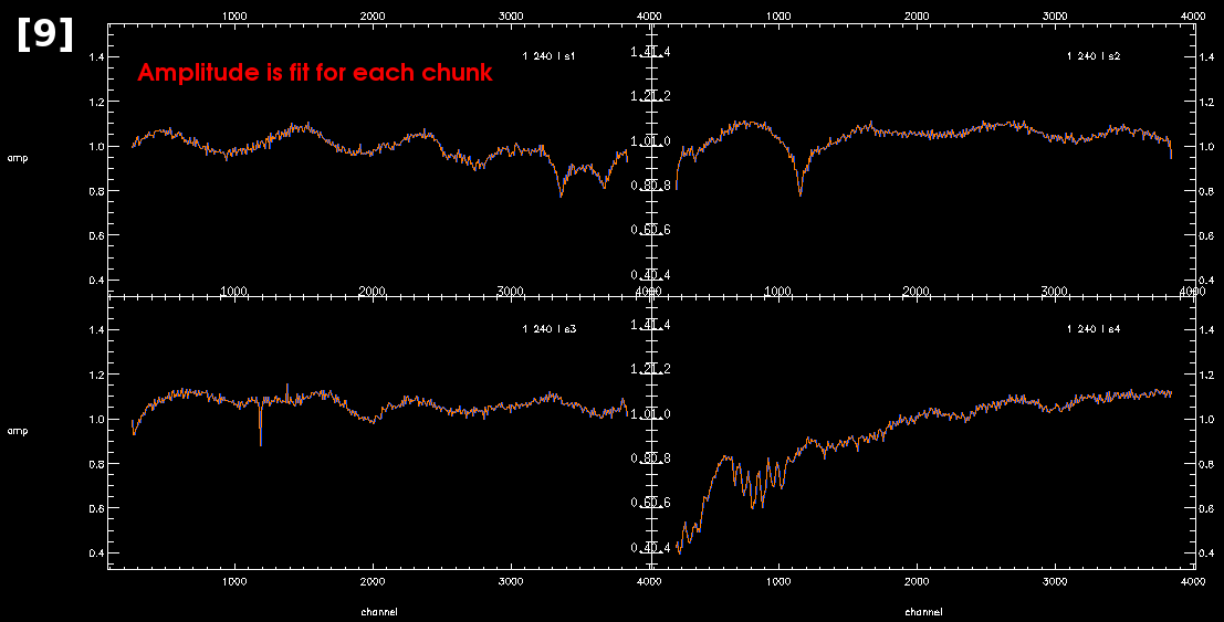
Apply the phase based bandpass first. For SWARM data use either no or minimal smoothing as there is a lot of detailed structure in the baseline. Note that the pass_cal command treats each sideband (and receiver) independently.
  Check: Found a total of            6  different sources in the data set.
  Set which sources will be used as calibrators and set the calibrator fluxes
  The flux should be in Jy at the frequency of the observation
  These are the sources and their current passband codes
  name:  0449+113           passband cal: NO
  name:  Science            passband cal: NO
  name:  0510+180           passband cal: NO
  name:  3c84               passband cal: YES
  name:  uranus             passband cal: NO
  name:  3c279              passband cal: YES
  Enter source and new cal code. eg: 3C273 YES
  or hit Return if all the sources are correctly specified
At this stage there is the option to accept the sources it suggests or add/remove any. Usually the bandpass calibrator(s) is identified as such in the software (and listed as YES) but not always. Add or remove sources by typing 3C273 YES or 0449+113 NO. Once it has generated a solution it will create a plot of the fits [8]. Right-click through the solutions for each baseline. After exiting the plot window it will prompt to apply the suggested solution to all other sources. If pass_cal fails reporting insufficient flux, try adding more sources to the list (if suitable ones are available), or increasing the 'preavg' value to boost the signal-to-noise.
Note the ntrim and preavg values have been scaled to account for this data having been rebinned by 4. For unbinned data use 1300 and 32 respectively. | 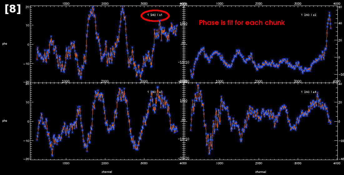
|
|
(8) Save the data
Select all unflagged data, regenerate the continuum and save in MIR format. It is important to save the dataset before starting flux measurement as the phases will be irreversibly disrupted.
| |
|
(9) Flux measurement
Make sure the data have been saved!
Do this section separately for each receiver and sideband.
Select all the calibrator sources and one of the sidebands.
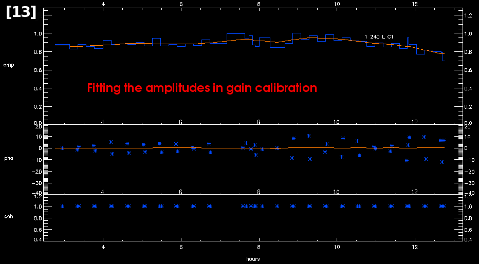
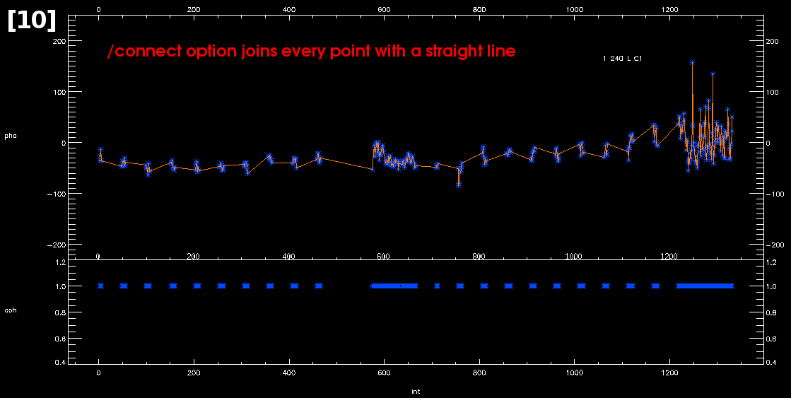
Apply the gain_cal in phase first with the /connect option to force the phases to zero for every scan [10]. The /non-point option takes into account the size of planets, on some baselines resolved planets may have a phase of ±180°.
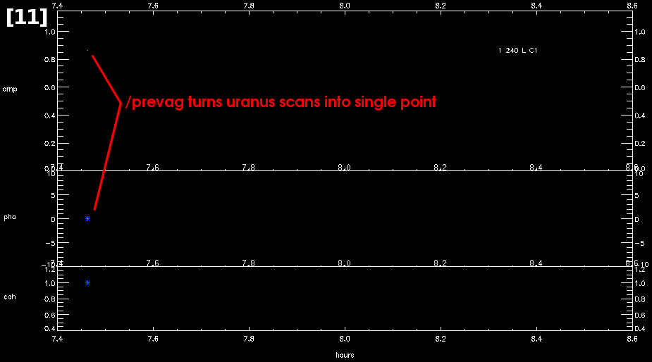
Next run amplitude based gain_cal [11]. Here, only say YES to the flux calibrator (usually a planet). Using the /non-point option it will retrieve its flux. Note that if your flux calibrator is not a planet or moon, you can provide the flux when prompted - e.g. mwc39a yes 1.8. This command will scale every source by the level required to make the flux calibrator match its expected flux.
    : all no
    : uranus yes
Note: the task sma_flux_cal performs a similar task to the amplitude gain calibratiom above. Now measure the resulting fluxes of the gain calibrators. The conditions (pointing/opacity/system) should be as similar as possible between the flux calibrator used to scale the data in the previous step, and the gain calibrator whose flux you are now calculating. To achieve this there are a couple of options available. Either select only scans taken close in time to the flux calibrator, or select only scans taken at a similar elevation. Sometimes only one of these options is available to you. The pointing model is less reliable at very high and low elevations so it always worth removing any elevation extremes (<30° and >70°). To choose scans close in time first plot the continuum with x as integration number, then select integration within an hour or two of the flux calibrator (here the first 200 scans).
To chose scans that are at a similar elevation use the result command (note that 'select' is just a wrapper for 'result=dat_filter'). Do not use the /reset option here or you will lose any previous selections (calibrators only, upper sideband, first 200 integrations).
Now measure the calibrated flux with flux_measure. It will return either vector or scalar values for each source included in the selection. (Vector terms adjust for phase noise so the amplitudes will be slightly lower).
For comparison here are the result for scalar average.
 Scalar average:
  #   Source   Flags   Nscans  Flux(Jy)   SNR    meantime    REAL       IMAG
    0449+113            122    0.3836     313      8.02      0.3791      0.0001
    0510+180             81    1.4383     407      8.07      1.4371     -0.0001
        3c84             14    8.7524     644      7.93      8.7523     -0.0001
       3c279             98    6.9338     508     13.18      6.9313     -0.0021
If the flux calibrator is included in the list you will see the scalar value for it will be the flux it was scaled to in the amplitude gain calibration step [11]. Now repeat for the lower sideband. |
|
|
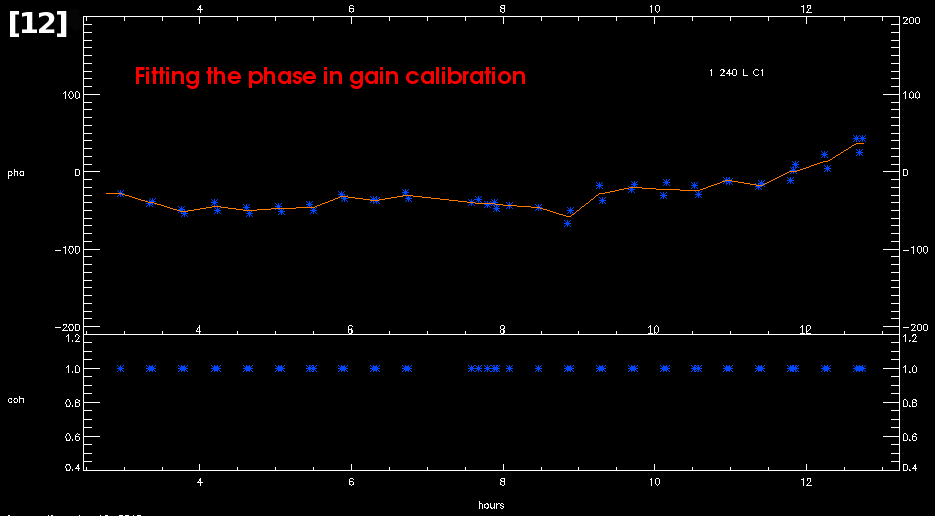
(10) Gain calibration on the restored data
With known fluxes for the gain calibrators, restore the previously saved file and perform time based gain calibration.
Select just the science and gain calibrator sources along with the sideband you are going to apply the corrections to first.
Apply the phase based gain_cal using /preavg and /connect [12]. The /connect option forces all the phases to 0 for the selected gain calibrators.
   : 0449+113 yes
   : 0510+180 yes
   : 0449+113 yes 0.3791
   : 0510+180 yes 1.4371
Now select the lower sideband data and re-run the gain_cal task to apply those corrections. |
|
|
(10) Apply the Doppler tracking error fix
Data taken between April 4th, 2011 and April 3rd, 2019 were affected by an error related to Doppler-tracking of data, which will affect spectral line measurements of features smaller than 1 km/sec in width. The effect is extremely small for most tracks, however the MIR task 'uti_hayshft_fix' can be used to make the correction.
|
|
|
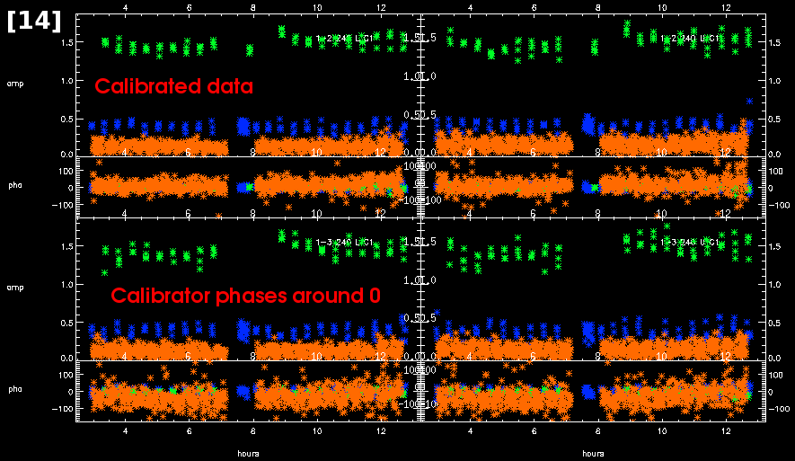
(11) Save the calibrated data
Reselect all the data
Have a final check of the calibrated dataset [14].
Then save the data in MIR format.
Export continuum and spectral data to MIRIAD.
Save the data in uvfits format to be read by CASA.
|
 |