Correction for System Temperature

Corrections for system temperature are carried out offline. For the recent SMA data, the corrections for T$_{\rm sys}$ use smafix :

smafix vis=050911H30a_rx0.usb out=050911H30a_rx0.usb.tsys \
	device=/xs xaxis=time yaxis=systemp nxy=2,4 \
	options=tsyscorr

Here, 050911H30a_rx0.usb is the Miriad formated data that is directly converted from SMA archival data and 050911H30a_rx0.usb.tsys is the output file which has been applied for T$_{\rm sys}$ to the fringe amplitude of the visibility.

For the older SMA data, since bad stablity of the total power detectors in T$_{\rm sys}$ measurements, the values of system temperature were corrupted. a repair for the corrupted T$_{\rm sys}$ measurements might be required prior to applying the T$_{\rm sys}$ corrections to the visibility data. smafix provides features for fixing bad T$_{\rm sys}$ measurements.

For old SMA archival data, here is a recommended procedure for T$_{\rm sys}$ correction in Miriad :

1. Polynomial Fit to T$_{\rm sys}$ and Apply T$_{\rm sys}$ Correction

smafix% inp
Task:   smafix                      
  vis    = gc_rx1.lsb           % name of the visibility 
                                  data file;
  out    = gc_rx1.lsb.tsys      % name of output file;
  device = /xs                  % pgplot device,X-windows 
                                  here;
  xaxis  = time                 % time in xaxis;
  yaxis  = systemp              % system temperature in 
                                    yaxis;
  nxy    = 2,4                  % 2 plots in xaxis and 
                                  4 in yaxis; 
  yrange = 100,1500             % plot range from 100 to 
                                  1500 in yaxis;
  dofit    = 2                  % polynomial fit;
  options  = tsyscorr,dosour,tsysswap       
                                % apply tsys corrections, 
                                  do source based fitting,
                                  replace the raw Tsys with 
                                  fitted values.

Figure: This plot shows a source-based second order polynomial fit to the antenna-based T$_{ \rm sys}$ as function of time for 8 antennas.

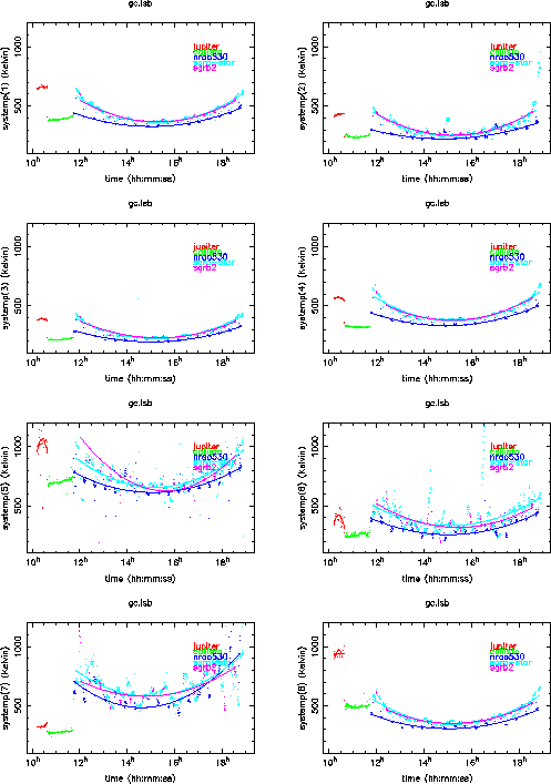A few fitting options have been provided to derive the T$_{\rm sys}$ corrections. Fig.2.1 shows a plot of antenna-based system temperature. Each panel stands for one antenna. A second order source-based polynomial fit to T$_{\rm sys}$ (solid lines) are carried out in order to get rid of the bad T$_{\rm sys}$ measurements. If options=tsyscorr, then the polynomial curves are replaced in the correctionis for system temperature. Careful users might like to check up the polynomial curves. The fitted T$_{\rm sys}$ is stored as a variable systmp in the uv data in the defualt options. If options=tsysswap, the fitted T$_{\rm sys}$ will swap with the orignal T$_{\rm sys}$, i.e. the fitted T$_{\rm sys}$ is stored as a variable systemp and the original T$_{\rm sys}$ goes to variable systmp.

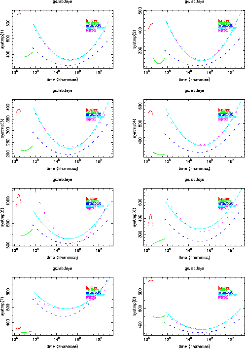
2. Check and Plot Fitted T$_{\rm sys}$

One can plot systmp or systemp using varplt or smavarplt (the sources are coded in different color; see Fig. 2.2):

smavarplt% inp
Task:   smavarplt
  vis      = gc_rx1.lsb.tsys
  device   = /xs
  xaxis    = time
  yaxis    = systemp       % the variable for fitted Tsys
  nxy      = 2,4

Figure: The ploynomial fit to system temperature is plotted. Each panel stands for each antenna. It is worth to mention that other Miriad tasks such as invert, smamfcal will use the variable values of systemp to calculate the variance of the data and the sensitivity weight in imaging and calibration.

3. Replacement and Flagging of Corrupted T$_{\rm sys}$

Occationally, an antenna might be corrupted in T$_{\rm sys}$ measurements. Users can choose a good antenna in T$_{\rm sys}$ measurements from the rest of the antennas to replace the bad antenna. The keyword bant in smafix can specify the id of the corrupted antenna and gant assigns a good antenna to replace the bad one. Here is a usage:

 Task:   smafix
  vis      = gc_rx1.lsb
  out      = gc_rx1.lsb.tsys
  device   = /xs
  xaxis    = antel
  yaxis    = systemp
  nxy      = 2,4
  bant     = 4                    % ant 4 is bad.
  gant     = 1                    % Tsys values of the good ant 1
                                    will replace those of ant 4.
  dofit    = 2
  options  = tsyscorr,dosour,tsysswap

Alternatively, the systemp values of ``bad antennas'' can be replaced with those of a good antenna without performing polynomial fitting:

 Task:   smafix
  vis      = visdata
  out      = visdata.tsys
  device   = /xs
  xaxis    = time 
  yaxis    = systemp
  nxy      = 2,4
  bant     = 1,8                  % ants 1, 8 are bad.
  gant     = 3                    % Tsys values of the good ant 3
                                    will replace those of ants 1, 8.

If only a few data points are corrupted, one may use smacheck to flag the data outside a specified range for the T$_{\rm sys}$ or other variables. By default, smafix will only take the unflagged (good) data in fitting, plotting and correction. There is an options of all to allow to use all (flagged and unflagged) data in the T$_{\rm sys}$ correction.