LINEAR REGRESSION BETWEEN 230/690 GHz PHASES

varfit is to analyse the correlations of antenna gains and uv-variables. varfit fits the following:

                    yaxis = slope *  xaxis +  intercept
                 D(yaxis) = slope * D(xaxis) + intercept

where D() is the difference between succesive samples, xaxis, yaxis are the uv variables from single uvfiles. In addition, varfit provides an option of regression for the phases derived from the gains of two uvfiles. If either axis is an antenna gain, then selfcal must be run first and the axes are sampled at the interval used in selfcal. For linear regression between the two phase solutions, the setup in the selfcal for the two simultaneously sampled data files needs identical. The rms and correlation coefficient are listed for each antenna.

varfit is a useful tool for analysis of the data obtained from observations at 230/690 GHz, simultaneously. An exmaple is shown to do linear regression between the phases derived from 230 and 690 GHz data sets based on the observations of Ceres on Feb 18, 2005 during the 690 GHz campaign. Ceres, $\sim$0.5 arcsec in size, was observed for 3.5 hrs at both lsb and usb. Here is the procedure to extract data from the raw SMA archival data:

1. Loading data:

\rm -r miriad050218_230_rx0.lsb
smalod in=/home/miriad/SMAdata/050218_04:23:14/ out=miriad050218_230 rxif=0 \
        sideband=0 options=dospc rsnchan=, \
        nscans=0,
\rm -r  miriad050218_690_rx2.lsb
smalod in=/home/miriad/SMAdata/050218_04:23:14/ out=miriad050218_690 rxif=2 \
        sideband=0 options=dospc rsnchan=, \
        nscans=0,

2. Qvack the first integrations after switching source:

qvack vis=miriad050218_230_rx0.lsb interval=0.5 mode=source
qvack vis=miriad050218_690_rx2.lsb interval=0.5 mode=source

3. Uvsplit ceres data from the multi-source files:

uvsplit vis=miriad050218_230_rx0.lsb select='source(ceres)' options=nowindow
uvsplit vis=miriad050218_690_rx2.lsb select='source(ceres)' options=nowindow
rename the file names:
mv ceres.221381 ceres.221lsb
mv ceres.682534 ceres.682lsb

4. Uvplt the two data sets together:

uvplt vis=ceres.221lsb,ceres.682lsb axis=time,pha options=nocal,unwrap \
        device=/xs nxy=3,5

Figure: Phase1 at 221 GHz (black dots) and phase2 at 682 GHz (red dots) versus time are plotted for each of the baselines.

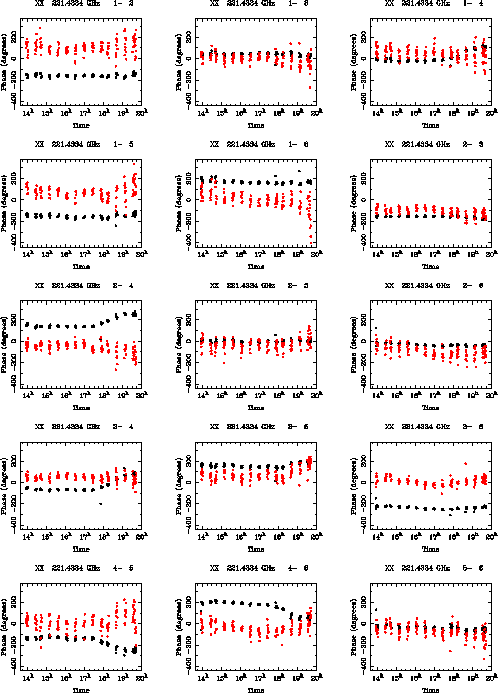5. Flag problematic data due to instruments:

There is a large phase drift on the baselines related to antenna 4 in the last 2.5 hrs of the observation at 221 GHz, which is apparently due to the instrument and mars the linear correlation between 221 GHz and 682 phases. To make the data sampling in the two files (221/682) identical, we flag all the antennas in the last 2.5 hrs for both files.

uvflag vis=ceres.221lsb select='time(17:27,23:00)' flagval=flag
uvflag vis=ceres.682lsb select='time(17:27,23:00)' flagval=flag

6. Selfcal to derive antenna-based phase:

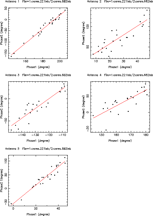
selfcal vis=ceres.221lsb interval=3 refant=6 line=chan,1,1,3072
selfcal vis=ceres.682lsb interval=3 refant=6 line=chan,1,1,3072

7. Varfit for linear regression of the 221/682 phases:

Input:

  Task:   varfit
  vis      = ceres.221lsb,ceres.682lsb
  xaxis    = time
  yaxis    = phase
  log      =
  device   = /xs
  nxy      = 2,3
  xrange   =
  yrange   =
  refant   = 6
  refant2  =
  options  = phareg

Report on screen:

Number of points= 24
Telescope: SMA       Longitude:   3.56959983 Latitude:   0.34599766

 yaxis = phase2 derived from gains of FILE1: ceres.682lsb
 xaxis = phase1 derived from gains of FILE2: ceres.221lsb

 yaxis = slope * xaxis + intercept
 ant   yaxis_ave   yaxis_rms   slope   intercept   rms-fit   correlation
 1 -32.2616653  51.0761375  3.11044097 -602.588867  9.25224018  0.983457565
 2  70.8661575  30.2317333  2.21507621  13.0970154  15.5836172  0.856906891
 3 -17.2317696  28.9356842  2.18647981  262.041107  11.3366861  0.920056641
 4  33.2323456  31.7655563  2.36979771 -359.516388  19.324564   0.793668747
 5  42.4374352  40.2758331  3.36416936 -55.4049721  11.4256344  0.958917618

 D(yaxis) = slope * D(xaxis) + intercept
 ant   yaxis_ave   yaxis_rms   slope   intercept   rms-fit   correlation
 1  8.04884434  50.8008919  3.14248133 -1.13375735  13.0757828  0.966306806
 2  9.50405884  30.7449551  2.18931246  2.78468132  20.3906422  0.748425245
 3  8.4316721   29.0480194  2.5807817   0.697852492 11.4700851  0.918738604
 4  6.80336809  32.7231979  2.22708535  1.3551662   19.3240604  0.807015002
 5  8.01961803  40.3351746  2.75186563  1.23834038  11.2498817  0.960317194

Plots the linear regression of 690/230 phases:

Figure: The linear regression between phase1 (221 GHz) and phase2 (682 GHz) derived from Miriad varfit for each antenna. Antenna 6 is the reference antenna.

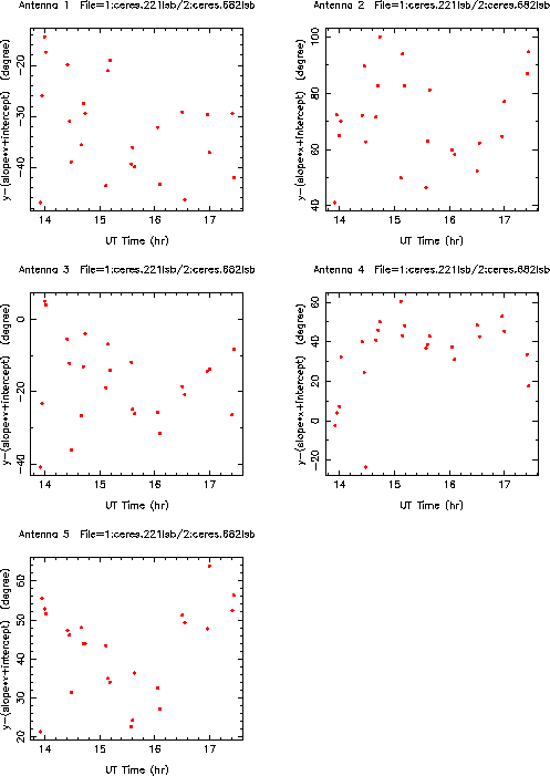
Plots the variation of the residual phase:

Figure: The residual phase (phase2_682 - slope*phase1_221 - intercept) as function of time calculated from varfit for each antenna. Antenna 6 is the reference antenna.