


Next: APPLY BANDPASS AND ANTENNA
Up: Normal Calibration Procedure
Previous: BANDPASS
We now process to calculations of the antenna gains using a phase calibrator.
In this testing program, NRAO 530 (a quasar) was used in the observation.
This source is a point source with flux density about 1.5-2 Jy at 335 GHz.
We use smamfcal
to solve for the antenna gains. A new keyword weight=1
is set, which allows to weight the visibility by 1/ ,
where
,
where  is the r.m.s. noise of the visibility data.
The solution interval of 1 minutes (which is smaller than the scan time
of 3 min). The solutions of the antenna gains can be smoothed or
polynomial interpolated afterwards. Here is a setup:
is the r.m.s. noise of the visibility data.
The solution interval of 1 minutes (which is smaller than the scan time
of 3 min). The solutions of the antenna gains can be smoothed or
polynomial interpolated afterwards. Here is a setup:
smamfcal  %inp
  Task:   smamfcal
  vis      = gc_rx1.lsb.tsys
  select   = source(nra*)       % select nrao530
  flux     = 2                  % flux density assumed
  refant   = 3                  % reference antenna
  interval = 1                  % solution interval
  weight   = 1                  % weight by 1/sigma**2
  options  = nopassol           % not solve for bandpass
The solutions of antenna gains can be inspected with smagpplt.
A setup for smagpplt
is shown below. There may be a few bad
points in the gain solutions. One may need to go back to smablflag
to do further data flagging. Or, one can use gplist
and gpedit
to reset bad point to (amp,phase)=(1,0). Alternatively, smagpplt
provides a nice feature for smoothing or polynomial fitting to the
antenna gains. An intermediate order of polynomial function may be
useful to fit the gain solutions in order to reduce the noise in
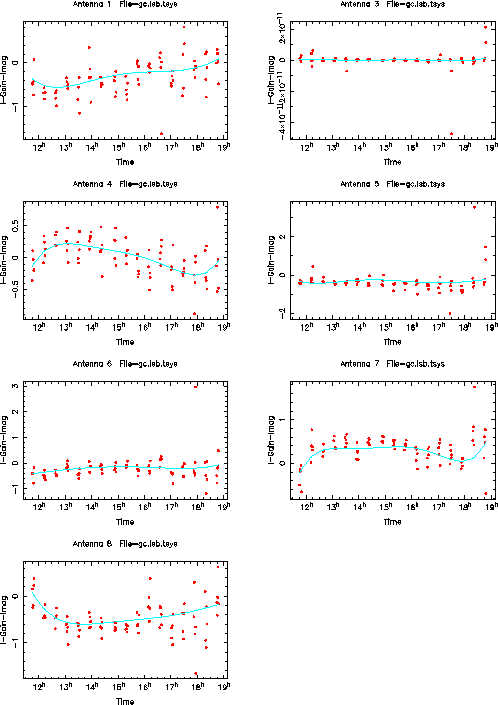
the gains. Figs. 3.3 and 3.4 show the plots of antenna-based gain
solutions (red points) in real and imaginary fit with the 5th order
polynomial curves (blue). One can replace the original gain solutions
with the polynomial fit by adding opolyfit to options or
options = gains,opolyfit. Note that in this observation,
antenna 2 showed odd values of the gain solutions in comparison
with other antennas. The problematic antenna may contaminate the data.
The antenna 2 has been flagged out.
One may get rid of the data related to problematic antennas prior to
further data processing. In most cases, the data from low S/N antennas
will mar the quality of images. If the baseline coverage is not a
concern, it would be wise to remove the bad quality data immediately.
smagpplt% inp
  Task:   smagpplt
  vis      = gc_rx1.lsb.tsys
  device   = /xs
  yaxis    = real,imag
  options  = gains,opolyfit
  polyfit  = 5
  nxy      = 2,4
Figure:
Antenna gain solutions in real (red dots) fitted with the 5th order polynomial (blue curves).
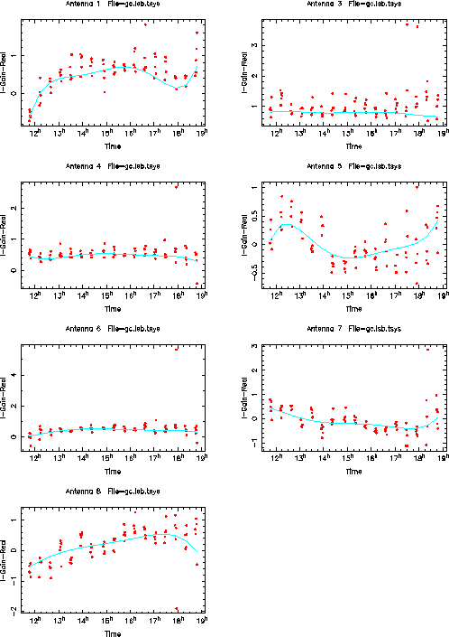 |
Figure:
Antenna gain solutions in imaginary (red dots) fitted with the 5th order polynomial (blue curves).
 |
Next: APPLY BANDPASS AND ANTENNA
Up: Normal Calibration Procedure
Previous: BANDPASS
Jun-Hui Zhao (miriad for SMA)
2012-07-09