1. Split the data into single-source files
Assuming the multiple source uv file 050911H30a_rx0.usb.tsys.bp.bl has been calibrated for bandpass. Two gain calibrators 2202+422 and 0102+584 were interleved. Here is the observing pattern of the target source interleaved with the two calibrators:
05SEP11:05:26:19.3 2202+422
05SEP11:05:32:00.0 n7538
05SEP11:05:42:50.5 2202+422
05SEP11:05:48:31.2 n7538
05SEP11:05:59:21.6 2202+422
05SEP11:06:05:02.3 3c454.3
05SEP11:06:15:47.6 2202+422
05SEP11:06:21:28.3 n7538
05SEP11:06:32:18.7 2202+422
05SEP11:06:37:59.4 n7538
05SEP11:06:48:49.9 0102+584
05SEP11:06:54:30.6 n7538
05SEP11:07:05:21.0 2202+422
05SEP11:07:11:01.7 n7538
05SEP11:07:21:52.2 0102+584
...
05SEP11:12:24:53.5 n7538
05SEP11:12:35:44.0 2202+422
05SEP11:12:41:24.7 n7538
05SEP11:12:52:15.1 0102+584
05SEP11:12:57:55.8 n7538
05SEP11:13:08:46.2 2202+422
05SEP11:13:14:27.0 n7538
05SEP11:13:25:17.4 0102+584
05SEP11:13:30:58.1 n7538
05SEP11:13:41:48.5 2202+422
05SEP11:13:47:29.2 n7538
05SEP11:13:58:19.7 0102+584
05SEP11:14:04:00.4 2202+422
The gain calibrators need to be splitted:
uvsplit vis=050911H30a\_rx0.usb.tsys.bp.bl \
        select='source(2202+422,0102+584)' \
	options=nowindows
mv 2202+422.230409 2202+422.gtest
mv 0102+584.230409 0102+584.gtest
The calibrators 2202+422 and 0102+584 are splitted into two separate
uv data sets and renamed the two single-source data files as
2202+422.gtest and 0102+584.gtest.
2. Solving for antenna gains from indvidual calibrators
Now, the antenna gains can be solved from the individual files using smamfcal:
smamfcal vis=2202+422.gtest refant=3 interval=1 \
       options=nopassol
smamfcal vis=0102+584.gtest refant=3 interval=1 \
       options=nopassol
Note that the default for the input Keyword flux is used here so that
the rms gain amplitude is set to 1 and no flux density scaling effect
is applied to the visibilities
in this process.
3. Merge the indvidual gain tables into a joint gain table
Then, the disjoint gain tables can be merged into a joint one, sorting into the ascending time order, with smagpplt:
smagpplt vis=2202+422.gtest,0102+584.gtest \
	device=/xw yaxis=amp,phase \
	options=gains,merge polyfit=8 \
        nxy=1,6
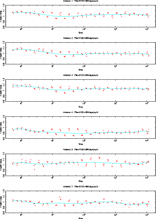
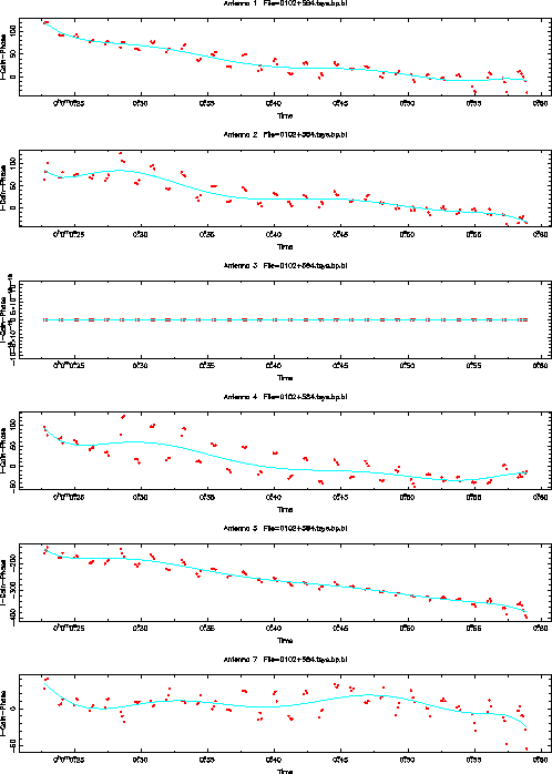
The merged gain table is placed under 0102+584.gtest, replacing
the old gain table. Fig.3.10 and Fig.3.11 shows the ampltidue
and phase curves computed from the merged gains (red dots).
For some reasons, the antenna gains derived from the two calibrators
show systematic offsets. The magnitude of the offsets varies with
antennas and time.
smagpplt
also provides orthogonal polynomial fits to the gains
in an order of polyfit=8 which can be specified by users.
The polynomial fits would be helpful to minimizing the systematic errors.
Users might wish to use the polynomial fits instead of the original
merged gains. Then, please go back to step 2 to recalculate
the antenna gains for 0102+584.gtest and redo smagpplt
with options=gains,merge,opolyfit instead of
options=gains,merge:
smagpplt vis=2202+422.gtest,0102+584.gtest \
        device=/xw yaxis=amp,phase \
        options=gains,merge,opolyfit polyfit=8 \
        nxy=1,6
The fitted gain table is placed under 0102+584.gtest.
The tradeoff in using the polynomial fits is that the detailed
structure in the original gains might be lost.
 |
 |
4. Gpcopy the merged gain table back to the multiple-source file
The mergered gain table in 0102+584.gtest is then copied back to 050911H30a_rx0.usb.tsys.bp.bl using gpcopy:
gpcopy vis=0102+584.gtest out=050911H30a_rx0.usb.tsys.bp.bl \
	mode=copy options=nopass