|
Abstract -
A procedure of SMA data reduction on CASA can be separated into three cycles, namely,
Pipeline SWARM data to CASA, Calibrations of SWARM data, and
Imaging calibrated SWARM data, consisting of sixteen steps:
- Step 0: Pipeline SMA data to CASA and apply online corrections -
- Step 1: Prepare for calibration -
- Step 2: Inspecting and editing data -
- Step 3: Set flux-density scale -
- Step 4: Solve for delay and bandpass -
- Step 5: Apply the delay and bandpass solution to the BP, CG, FL data1 -
- Step 6: Solve for complex gain -
- Step 7: Bootstrap flux-density scale from a reference source -
- Step 8: Apply calibration solutions to the data -
- Step 9: Examine and edit calibrated data -
- Step 10: Split calibrated multi-source data into single-source sets -
- Step 11: Examine the calibrated data with imaging -
- Step 12: Image continuum emission (MS-MFS) -
- Step 13: Identify spectral lines and construct image cubes -
- Step 14: Combine of different array data -
- Step 15: Convert CASA image to FITS -
This webpage provides a demostration for wSMA data reduction on CASA
after raw swarm data from
SMA data archive converted
to CASA format - measurementSet with the newly developed pipeline software SWARM2CASA
(1.0.5). The detailed usages of the pipeline are scripted in swarm2casa.csh,
discussed in Step 0. A CASA procedure for the calibration and imaging of SMA swarm data is discussed in the thirteen steps
(Step 1 - 13).
Step 14 provides an extra guideline
if two or more data sets taken in different array configurations need to be combined. Step 15 allows users to convert CASA
images to FITS format for analysis in other software packages.
The demonstration below uses SMA swarm data set 181002_03:55:28 of SMA project: 2018A-S005 with archived information:
PI                 - Tomasz Kaminski
Target             - CK Vul
RA (J2000)         - 19:47:38.07
Dec (J2000)        - 27:18:45.2
LO Freq (GHz)      - 340.8 (B), 340.8 (A) (B: 400 rx , A: 345 rx)
N-bsln             - 28(B), 28(A)
Angular resolution - 2.51"(B), 2.57"(B)
Time               - 227 min
_____________________________________
1The calibrator codes BP, CG, FL stand for bandpass, complex gain, and flux density.
Pipeline SWARM to CASA -
Step 0: Pipeline SMA data to CASA and apply online corrections -
- Input SMA swarm data: 181002_03:55:28
-
Usage of C-shell script: swarm2casa.csh
- Purpose with OPTIONS = 2:
- convert SMA swarm data into CASA measurementSet
- apply Tsys corrections and online error flagging
- Output of CASA measurementSet: SMA181002.ms
Calibrations of SWARM data -
############################################
#define variables for swarm data reduction #
############################################
datain   = 'SMA181002'
inttime  = 5.2   #~5.16
dinttime = 10.4
tinttime = 16
qsecond  = 30.0
allspw   = '0~15'
allspw1  = '0~15:512~15871'
allspw2  = '0~15:1024~15359'
quadspw  = '0,4,8,12'
nchspw   = 16384
nchnew   =  1792
width0   =    1
width1   =    2
width2   =    4
width3   =    8
width4   =   16
width5   =   32
width6   =   64
width7   =  128
avgchan0 =   '1'
avgchan1 =   '2'
avgchan2 =   '4'
avgchan3 =   '8'
avgchan4 =  '16'
avgchan5 =  '32'
avgchan6 =  '64'
avgchan7 = '128'
#############################################
#user's setup below -                       #
#############################################
#
# Note for import data -
# the input measurementSet must be created via the swarm2casa path
#
#prefix of swarm measurementSet -
datain   = 'SMA181002'
#full name of swarm measurementSet -
datainms = 'SMA181002.ms'
#number of channels to average -
bw       = width3
#define source code -
CG = '0'   #complex gain calibrator
T1 = '1'   #primary target
T2 = '2'   #secondary target
FL = '3'   #flux density scale calibrator
BP = '4~5' #bandpass calibrator
BP2 =  '3' #secondary bandpass calibrator
#define source name -
BPname = '3c84'
BP2name ='Neptune'
CGname = '2015+371'
T1name = 'CKVul'
T2name = 'mwc349a'
FLname = 'Neptune'
#define reference antenna -
rant = '5'
#
Step 1: Prepare for calibration-
CASA tasks:
     listobs
     plotants
     split
Usage of CASA-python-script module -
Listobs output -
Table 1: Source/Field information -
| Source (Field) information reported from CASA listobs |
|---|
| ID |
Code# |
Name |
RA |
Decl |
Epoch |
SrcId |
nRows |
| 0 | CG | 2015+371 | 20:15:28.729248 | +37.10.59.50928 | J2000 | 0 | 84672 |
| 1 | T1 | CKVul | 19:47:38.072662 | +27.18.45.16479 | J2000 | 1 | 206080 |
| 2 | T2 | mwc349a | 20:32:45.543365 | +40.39.36.61743 | J2000 | 2 | 43008 |
| 3 | FL/BP2$ | Neptune | 23:04:10.625610 | -07.03.08.71422 | J2000 | 3 | 8960 |
| 4~5 | BP* | 3c84/0319+415 | 03:19:48.160229 | +41.30.42.10510 | J2000 | 4/5 |
3696/66640 |
________________
*Check listobs_log for the issue of source ID and spw mix-up
#Note for Code:
BP - bandpass
CG - complex gain
T1 - Target source
T2 - Secondary target source for examing calibration
FL - Flux density scale calibrator
$ BP2 = FL - Neptune is an option to be used to solve for bandpass;
however, Neptune's spectrum presents a significant broad spectral feature and is not suitable for bandpass calibration but is good for examining bandpass calibration.
Table 2: Correlator/Frequency configuration, original -
|
Spectral Windows: (16 unique spectral windows and 1 unique polarization setups) |
|---|
| SpwID |
Name |
#Chans |
Frame |
Ch0(MHz) |
ChanWid(kHz) |
TotBW(kHz) |
CtrFreq(MHz) |
Corrs |
| 0 | none | 16384 | LSRK | 336962.794 | -139.648 | 2288000.0 | 335818.8637 | XX |
| 1 | none | 16384 | LSRK | 332663.081 | 139.648 | 2288000.0 | 333807.0108 | XX |
| 2 | none | 16384 | LSRK | 332962.801 | -139.648 | 2288000.0 | 331818.8710 | XX |
| 3 | none | 16384 | LSRK | 328663.088 | 139.648 | 2288000.0 | 329807.0181 | XX |
|
4 | none | 16384 | LSRK | 344963.088 | -139.648 | 2288000.0 | 343819.1576 | XX |
|
5 | none | 16384 | LSRK | 340663.374 | 139.648 | 2288000.0 | 341807.3045 | XX |
|
6 | none | 16384 | LSRK | 340963.095 | -139.648 | 2288000.0 | 339819.1646 | XX |
|
7 | none | 16384 | LSRK | 336663.380 | 139.648 | 2288000.0 | 337807.3104 | XX |
|
8 | none | 16384 | LSRK | 344663.061 | 139.648 | 2288000.0 | 345806.9907 | XX |
|
9 | none | 16384 | LSRK | 348962.774 | -139.648 | 2288000.0 | 347818.8435 | XX |
|
10 | none | 16384 | LSRK | 348663.053 | 139.648 | 2288000.0 | 349806.9837 | XX |
|
11 | none | 16384 | LSRK | 352962.767 | -139.648 | 2288000.0 | 351818.8367 | XX |
|
12 | none | 16384 | LSRK | 352663.354 | 139.648 | 2288000.0 | 353807.2839 | XX |
|
13 | none | 16384 | LSRK | 356963.067 | -139.648 | 2288000.0 | 355819.1372 | XX |
|
14 | none | 16384 | LSRK | 356663.347 | 139.648 | 2288000.0 | 357807.2771 | XX |
|
15 | none | 16384 | LSRK | 360963.060 | -139.648 | 2288000.0 | 359819.1302 | XX |
- Plot antenna array -
 Fig. 1: Antenna array. Click the figure for enlargement.
Split & bin data -
Listobs output (binned data) -@
_____________________________________
@Note: the original spectral data are binned with
bw = width3, or vector-averaging 8 channels to produce a new channel width of 1.117188 MHz,
which provides an adequate velocity resolution (1 km/s) for this project.
Step 2: Inspecting and editing data -
CASA tasks:
plotms
Usage of CASA-python-script module -
- Plot uv-coverage -
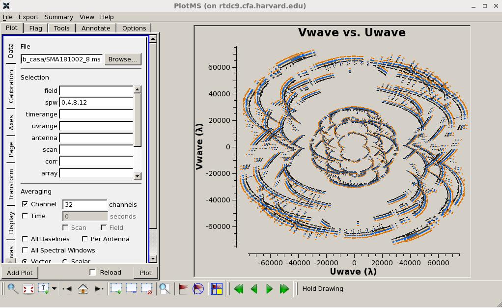 Fig. 2: uv-coverage (spw 0,4,8,12) (all fields). Click the figure for enlargement.
- Plot elevation coverage -
 Fig. 3: Elevation coverage including all field (0~5).
Black: 0 CG 2015+371; Red: 1 T1 CKVul;
Orange: 2 T2 mwc349a;
Green: 3 FL Neptune;
Blue/Brown: 4~5 BP* 3c84/0319+415.
Click the figure for enlargement.
Fig. 3: Elevation coverage including all field (0~5).
Black: 0 CG 2015+371; Red: 1 T1 CKVul;
Orange: 2 T2 mwc349a;
Green: 3 FL Neptune;
Blue/Brown: 4~5 BP* 3c84/0319+415.
Click the figure for enlargement.
- Plot fringe amplitude vs time -
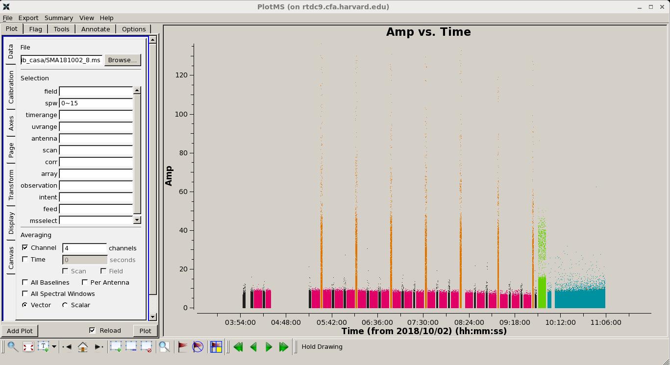 Fig. 4: Fringe amplitude vs time after flagging a few high-amplitude spikes in the inspect&editing cycle (pre-calibration).
Black: 0 CG 2015+371; Red: 1 T1 CKVul;
Orange: 2 T2 mwc349a;
Green: 3 FL Neptune;
Blue/Brown: 4~5 BP* 3c84/0319+415.
Click the figure for enlargement.
Fig. 4: Fringe amplitude vs time after flagging a few high-amplitude spikes in the inspect&editing cycle (pre-calibration).
Black: 0 CG 2015+371; Red: 1 T1 CKVul;
Orange: 2 T2 mwc349a;
Green: 3 FL Neptune;
Blue/Brown: 4~5 BP* 3c84/0319+415.
Click the figure for enlargement.
Step 3: Set flux density scale -
CASA tasks:
setjy
Usage of CASA-python-script module -
Note: FL is Neptune that is used to set the flux-density scale with the model standard:
Butler-JPL-Horizons 2012
Setjy output -
Table 3: Results of setjy -
|
FL is Neptune that is used to set the flux-density scale with the model standard:
Butler-JPL-Horizons 2012 |
|---|
| Reference source |
Specral window |
Flux density |
Frequency |
|
Neptune: | spw0 | Flux:[I=25.854,Q=0.0,U=0.0,V=0.0] +/- [I=0.0,Q=0.0,U=0.0,V=0.0] Jy | @ 336.82GHz |
|
Neptune: | spw1 | Flux:[I=25.692,Q=0.0,U=0.0,V=0.0] +/- [I=0.0,Q=0.0,U=0.0,V=0.0] Jy | @ 332.81GHz |
|
Neptune: | spw2 | Flux:[I=25.693,Q=0.0,U=0.0,V=0.0] +/- [I=0.0,Q=0.0,U=0.0,V=0.0] Jy | @ 332.82GHz |
|
Neptune: | spw3 | Flux:[I=25.361,Q=0.0,U=0.0,V=0.0] +/- [I=0.0,Q=0.0,U=0.0,V=0.0] Jy | @ 328.81GHz |
|
Neptune: | spw4 | Flux:[I=22.053,Q=0.0,U=0.0,V=0.0] +/- [I=0.0,Q=0.0,U=0.0,V=0.0] Jy | @ 344.82GHz |
|
Neptune: | spw5 | Flux:[I=25.447,Q=0.0,U=0.0,V=0.0] +/- [I=0.0,Q=0.0,U=0.0,V=0.0] Jy | @ 340.81GHz |
|
Neptune: | spw6 | Flux:[I=25.444,Q=0.0,U=0.0,V=0.0] +/- [I=0.0,Q=0.0,U=0.0,V=0.0] Jy | @ 340.82GHz |
|
Neptune: | spw7 | Flux:[I=25.854,Q=0.0,U=0.0,V=0.0] +/- [I=0.0,Q=0.0,U=0.0,V=0.0] Jy | @ 336.81GHz |
|
Neptune: | spw8 | Flux:[I=22.073,Q=0.0,U=0.0,V=0.0] +/- [I=0.0,Q=0.0,U=0.0,V=0.0] Jy | @ 344.81GHz |
|
Neptune: | spw9 | Flux:[I=25.307,Q=0.0,U=0.0,V=0.0] +/- [I=0.0,Q=0.0,U=0.0,V=0.0] Jy | @ 348.82GHz |
|
Neptune: | spw10 | Flux:[I=25.296,Q=0.0,U=0.0,V=0.0] +/- [I=0.0,Q=0.0,U=0.0,V=0.0] Jy | @ 348.81GHz |
|
Neptune: | spw11 | Flux:[I=27.476,Q=0.0,U=0.0,V=0.0] +/- [I=0.0,Q=0.0,U=0.0,V=0.0] Jy | @ 352.82GHz |
|
Neptune: | spw12 | Flux:[I=27.472,Q=0.0,U=0.0,V=0.0] +/- [I=0.0,Q=0.0,U=0.0,V=0.0] Jy | @ 352.81GHz |
|
Neptune: | spw13 | Flux:[I=28.462,Q=0.0,U=0.0,V=0.0] +/- [I=0.0,Q=0.0,U=0.0,V=0.0] Jy | @ 356.82GHz |
|
Neptune: | spw14 | Flux:[I=28.459,Q=0.0,U=0.0,V=0.0] +/- [I=0.0,Q=0.0,U=0.0,V=0.0] Jy | @ 356.81GHz |
|
Neptune: | spw15 | Flux:[I=29.146,Q=0.0,U=0.0,V=0.0] +/- [I=0.0,Q=0.0,U=0.0,V=0.0] Jy | @ 360.82GHz |
Step 4: Solve for delay & bandpass -
CASA tasks:
     plotms
     gaincal
     bandpass
     plotcal
Usage of CASA-python-script module -
Note: using the BP (3c84) to solve for delay.
- Plot delay corrections -
 Fig. 5: Antenna-based delay as function of time. The remaining delay shows a typical value of a few tens pico seconds,
quite small. Click the figure for enlargement.
Fig. 5: Antenna-based delay as function of time. The remaining delay shows a typical value of a few tens pico seconds,
quite small. Click the figure for enlargement.
Note: two options of solving for bandpass
- Option 1: 3c84 as defined early as a variable BP -
- Option 2: Neptune that was identified as flux density calibrator (FL) and also can be used as bandpass calibrator
(BP2) -
- Plot bandpass phase correction -

Fig. 6: Antenna-based phase soultions as function of time solvd for BP, which needs to be applied to the data while
solving for bandpass. Click the figure for enlargement.
OPTION 1 -
- Plot bandpass amplitude-

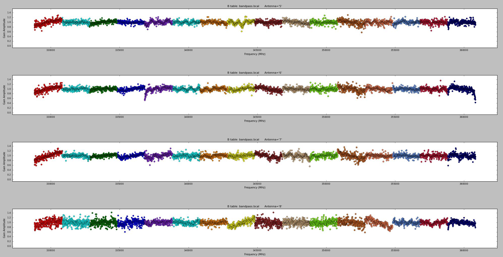 Fig. 7: Antenna-based bandpass solutions (amplitude) for option 1 (BP=3c84), solved with averaging every 16 channels. Top panel for antennas 1~4; bottom panel for
antenna 5~8. Click the figure for enlargement.
Fig. 7: Antenna-based bandpass solutions (amplitude) for option 1 (BP=3c84), solved with averaging every 16 channels. Top panel for antennas 1~4; bottom panel for
antenna 5~8. Click the figure for enlargement.
- Plot bandpass phase-
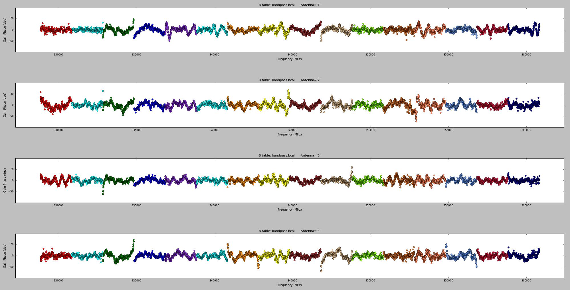
 Fig. 8: Antenna-based bandpass solutions (phase) for option 1 (BP=3c84), solved with averaging every 16 channels. Top panel for antennas 1~4; bottom panel for
antenna 5~8. Click the figure for enlargement.
Fig. 8: Antenna-based bandpass solutions (phase) for option 1 (BP=3c84), solved with averaging every 16 channels. Top panel for antennas 1~4; bottom panel for
antenna 5~8. Click the figure for enlargement.
OPTION 2 -
- Plot bandpass amplitude-
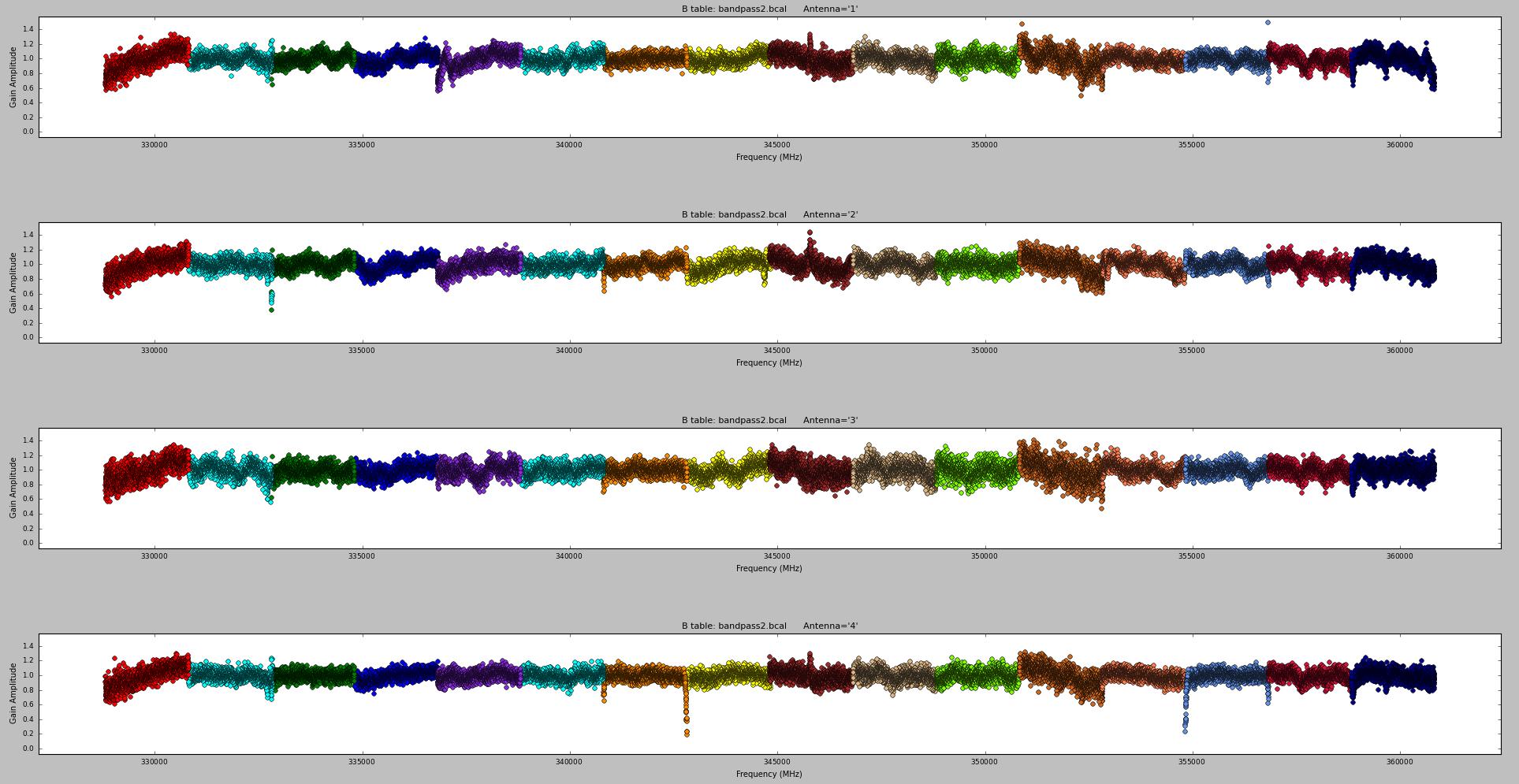
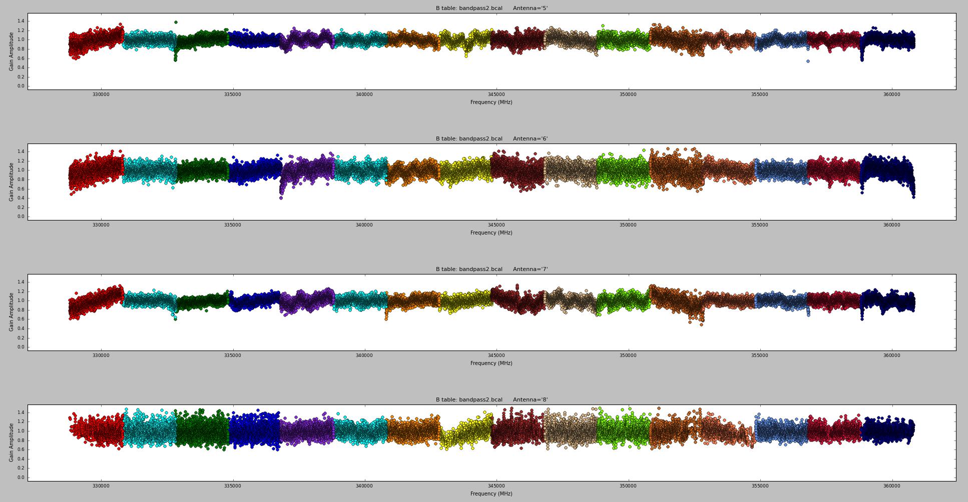 Fig. 9: Antenna-based bandpass solutions (amplitude) for option 2 (BP2=Neptune), solved with each channel. Top panel for antennas 1~4; bottom panel for
antenna 5~8. Click the figure for enlargement.
Fig. 9: Antenna-based bandpass solutions (amplitude) for option 2 (BP2=Neptune), solved with each channel. Top panel for antennas 1~4; bottom panel for
antenna 5~8. Click the figure for enlargement.
- Plot bandpass phase-
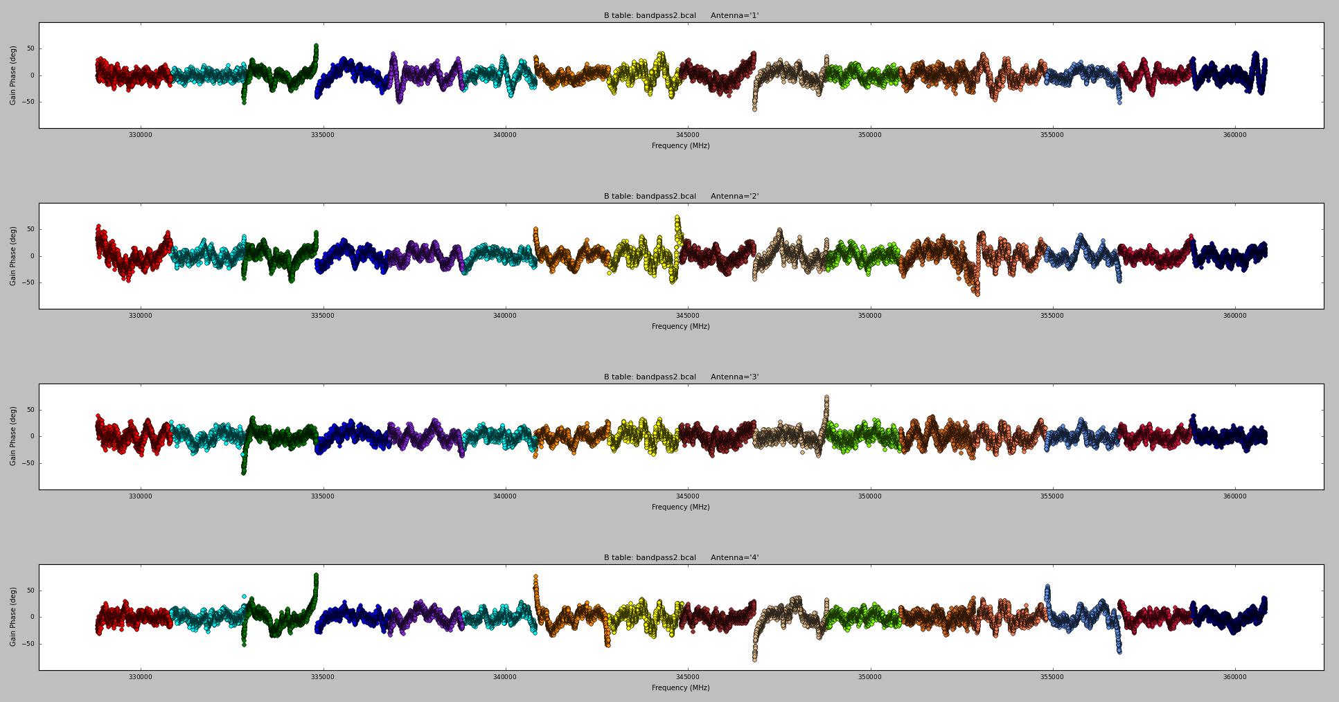
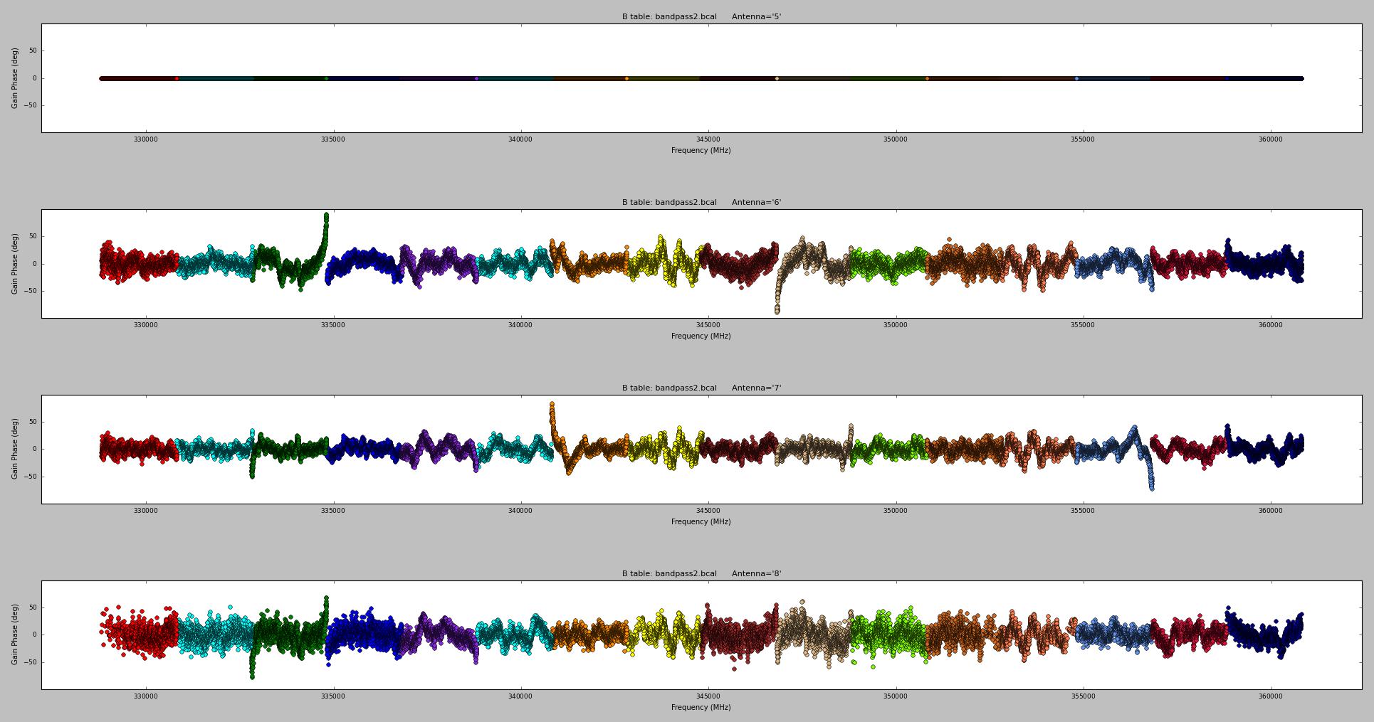 Fig. 10: Antenna-based bandpass solutions (phase) for option 1 (BP2=Neptune), solved with each channel. Top panel for antennas 1~4; bottom panel for
antenna 5~8. Click the figure for enlargement.
Fig. 10: Antenna-based bandpass solutions (phase) for option 1 (BP2=Neptune), solved with each channel. Top panel for antennas 1~4; bottom panel for
antenna 5~8. Click the figure for enlargement.
Step 5: Apply the delay and bandpass solution to the BP, CG, FL data -
CASA tasks:
     applycal
     plotms
Usage of CASA-python-script module -
Note: edting the data before next step
Step 6: Solve for complex gains -
CASA tasks:
     gaincal
     plotcal
Usage of CASA-python-script module:
Note: solving for complex gains for the calibrators FL, BP and CG prior to bootstrape the flux-density scale
- Plot phase solutions in integration-
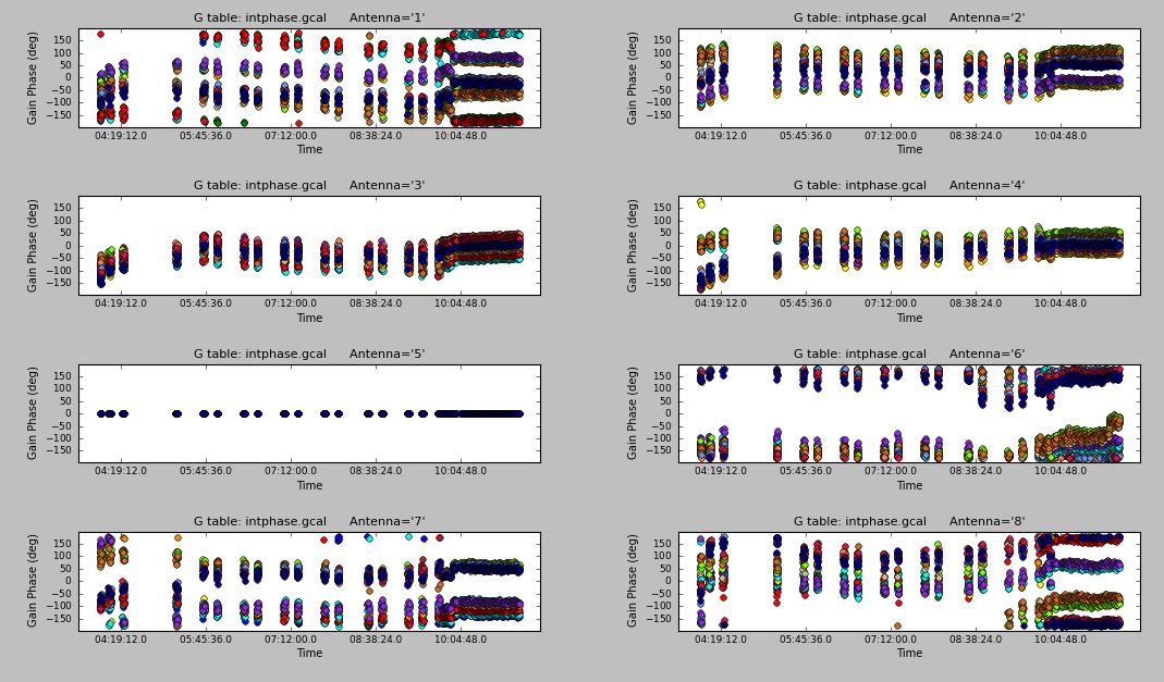 Fig. 11. Antenna-based phase solutions (integration) for the calibrators FL, BP and CG.
Click the figure for enlargement.
Fig. 11. Antenna-based phase solutions (integration) for the calibrators FL, BP and CG.
Click the figure for enlargement.
- Plot phase solutions in scan-
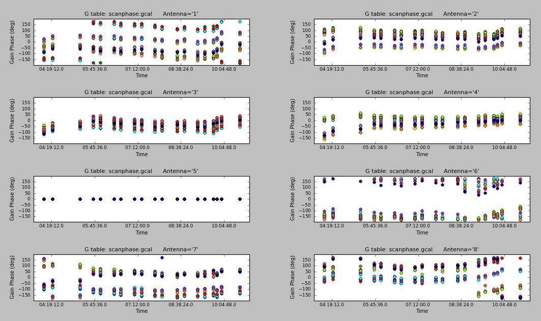 Fig. 12. Antenna-based phase solutions (scan) for the calibrators FL, BP and CG.
Click the figure for enlargement.
Fig. 12. Antenna-based phase solutions (scan) for the calibrators FL, BP and CG.
Click the figure for enlargement.
Step 7: Bootstrap flux-density scale from a reference source (FLname: Neptune) -
CASA tasks:
     fluxscale
Usage of CASA-python-script module:
Note: Report from CASA bootstraping
Table 4: A summary of flux density bootstraping -
|
Statistics of flux-density from the 16 spws |
|---|
| Calibrators |
Flux density and 1 σ uncertainty (Jy) |
Spectral index and 1 σ uncertainty |
Frequency(GHz) |
| 2015+371 | 0.857746 +/- 0.00692425 | -0.953203 +/- 0.304559 | 344.690 |
| 3c84 | 5.11449 +/- 0.0304287 | -1.08358 +/- 0.219112 | 345.289 |
Step 8: Apply calibration solutions to the data -
CASA tasks:
     fluxscale
Usage of CASA-python-script module:
Note: apply the calibrations to all the calibrators and target sources interested:
- 3c84 (BP),
- 2015+371 (CG),
- Neptune (FL),
- CKVul (T1), primary target
- mwc349a (T2), secondary target
Step 9: Examine and edit calibrated data -
CASA tasks:
     plotms
Usage of CASA-python-script module:
CG(2015+371) -
- Plot spectra -
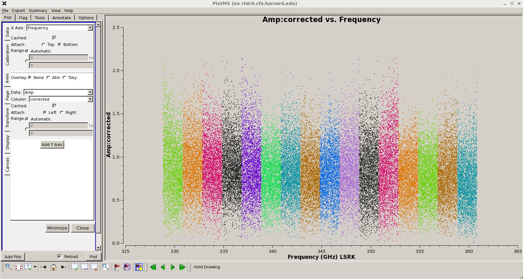
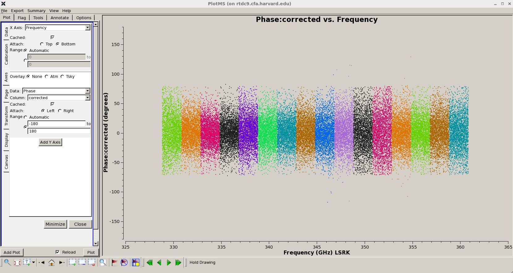 Fig. 13 Spetra of the gain calibrator (2015+371). Top: amplitude. Bottom: phase.
Click the figure for enlargement.
Fig. 13 Spetra of the gain calibrator (2015+371). Top: amplitude. Bottom: phase.
Click the figure for enlargement.
- Plot uv structure -
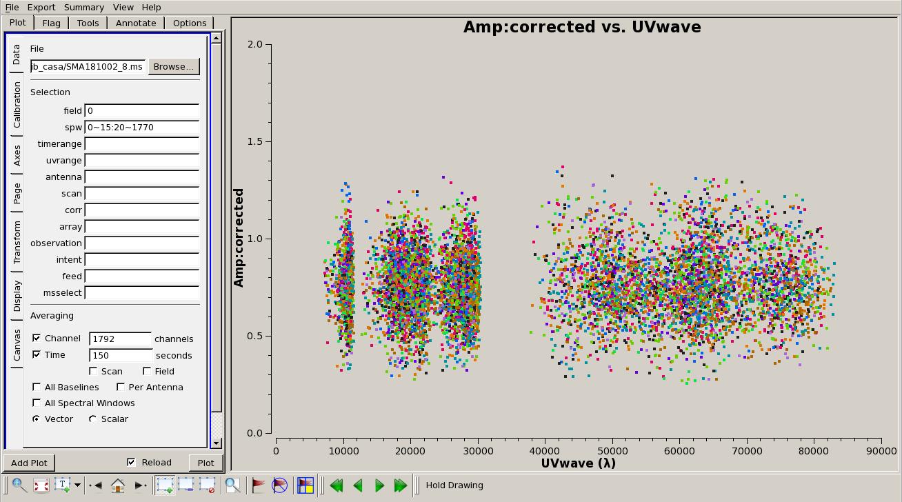 Fig. 14. UV structure of the gain calibrator (2015+371). Click the figure for enlargement.
FL(Neptune) -
- Plot spectrum -
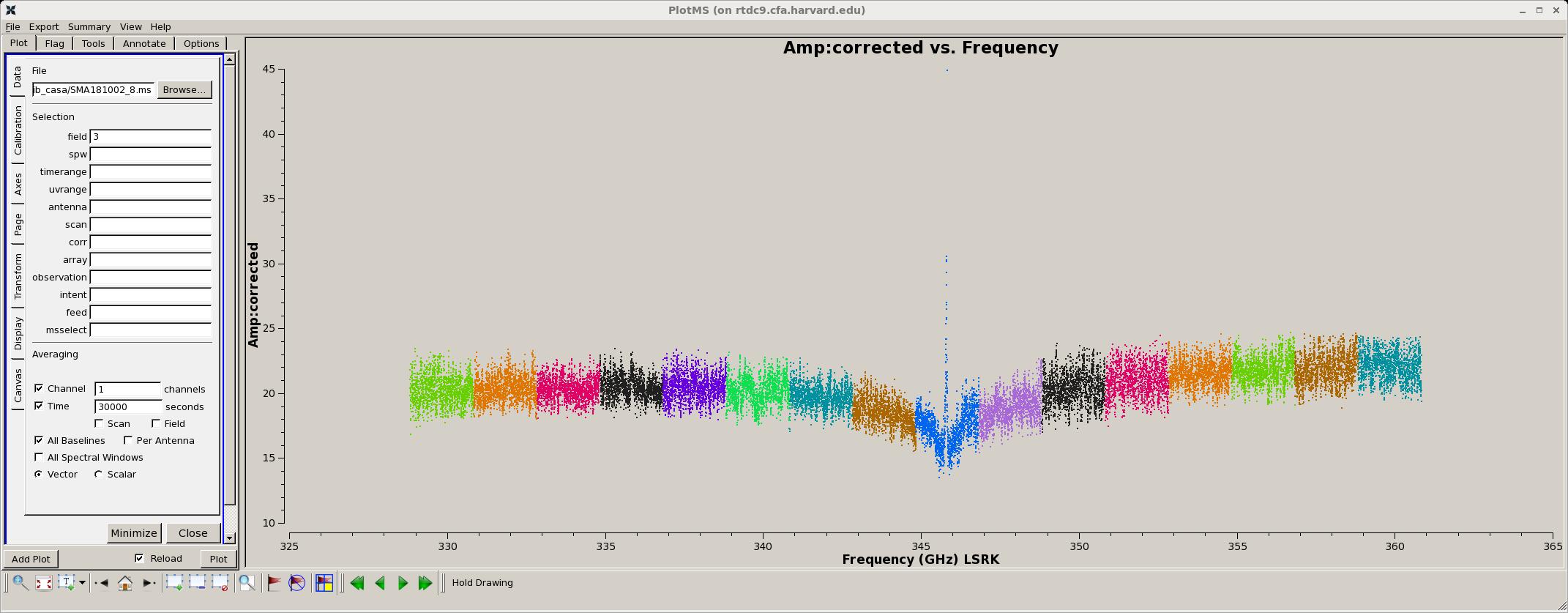 Fig. 15. Spetrum of the flux-density calibrator (Neptune). A broad absorption spectral feature,
centered in spw 8 at 345.7 GHz with a narrow emission spectral feature set in the absorption dip. Click the figure for enlargement.
Fig. 15. Spetrum of the flux-density calibrator (Neptune). A broad absorption spectral feature,
centered in spw 8 at 345.7 GHz with a narrow emission spectral feature set in the absorption dip. Click the figure for enlargement.
- Plot uv structure -
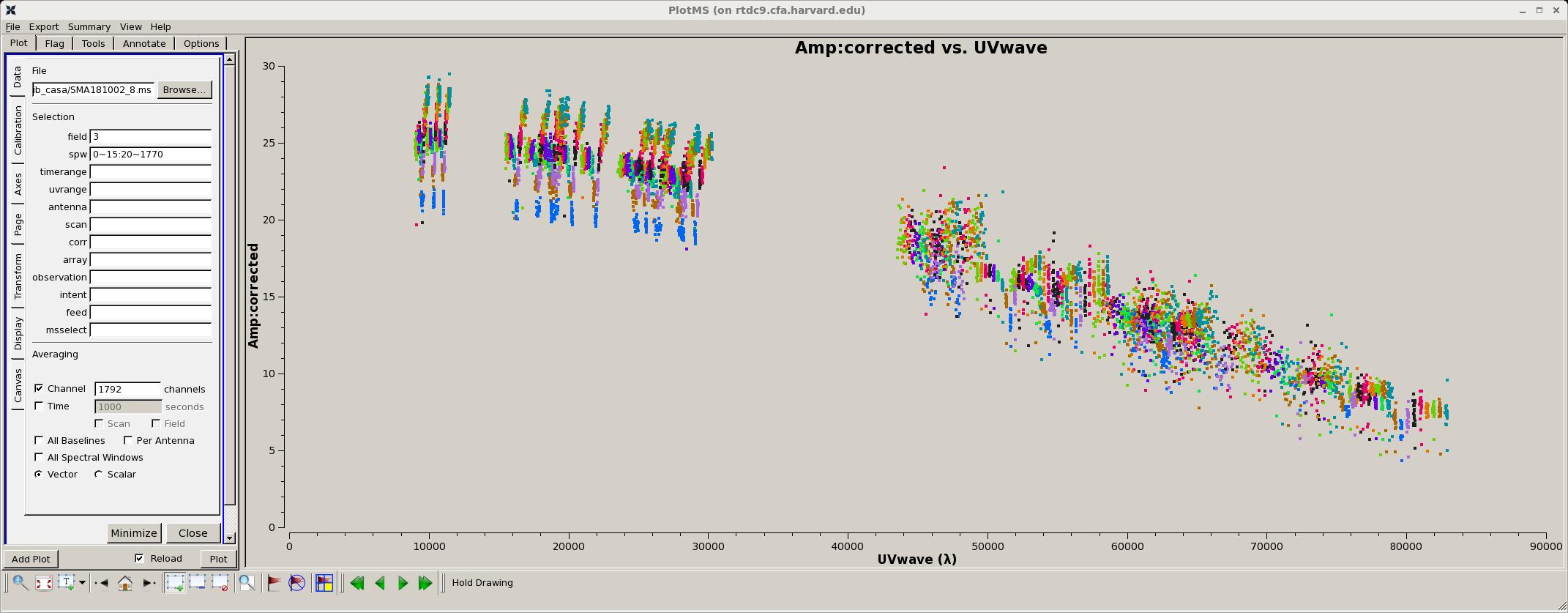 Fig. 16. UV structure of the flux-density calibrator (Neptune). Click the figure for enlargement.
BP(3c84) -
- Plot spectrum -
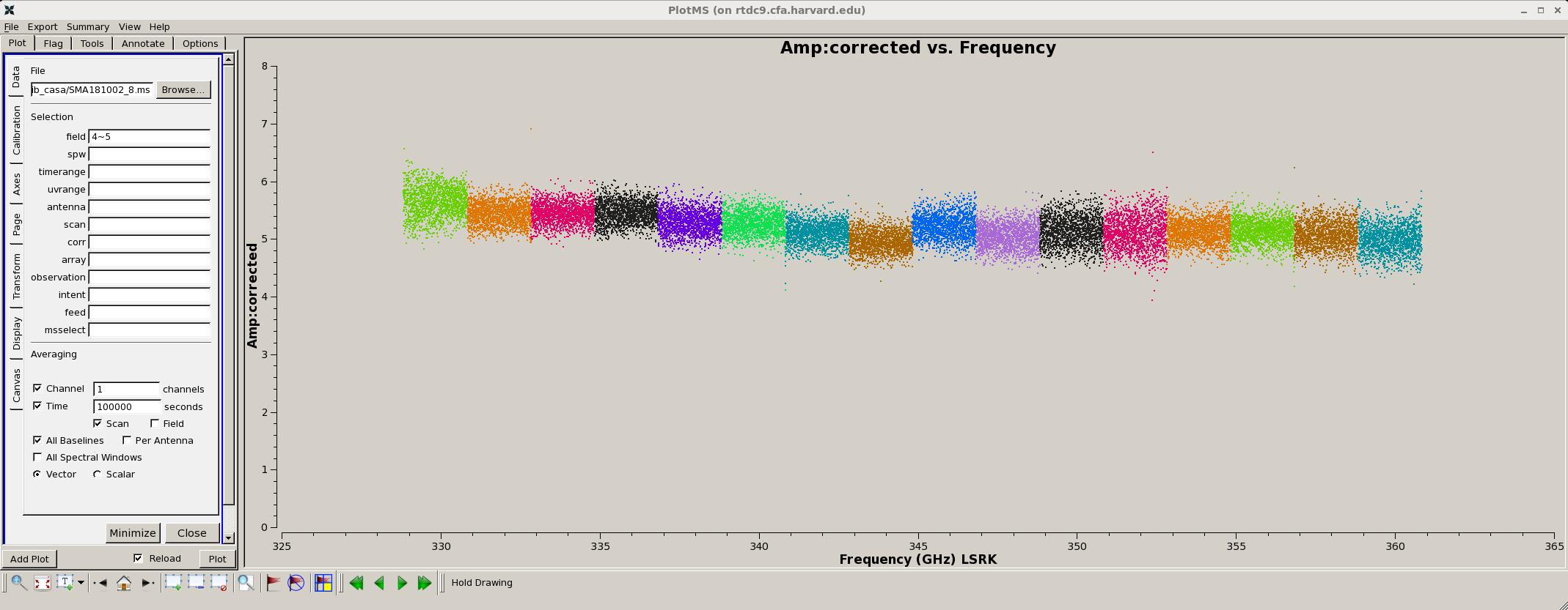 Fig. 17. Spetrum of the delay/bandpass calibrator (3c84) after applying the corrections.
Click the figure for enlargement.
Fig. 17. Spetrum of the delay/bandpass calibrator (3c84) after applying the corrections.
Click the figure for enlargement.
- Plot UV structure -
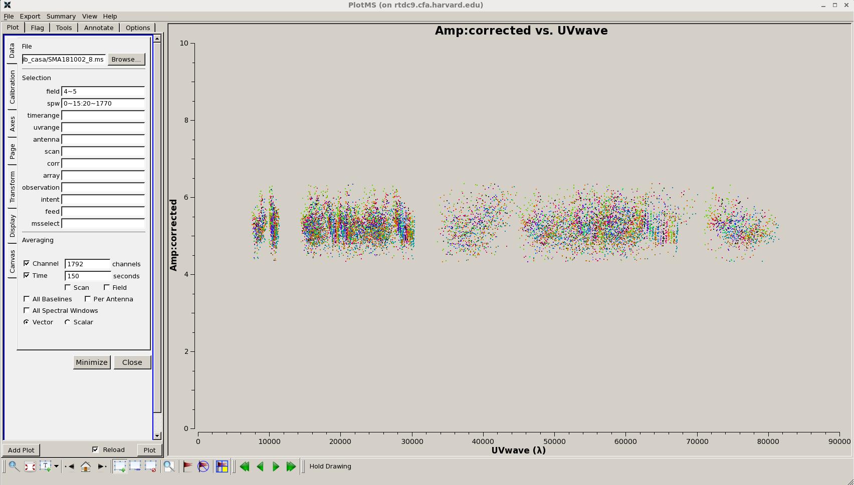 Fig. 18. UV structure of the bandpass calibrator (3c84). Click the figure for enlargement.
T2(mwc349a) -
- Plot spectra -
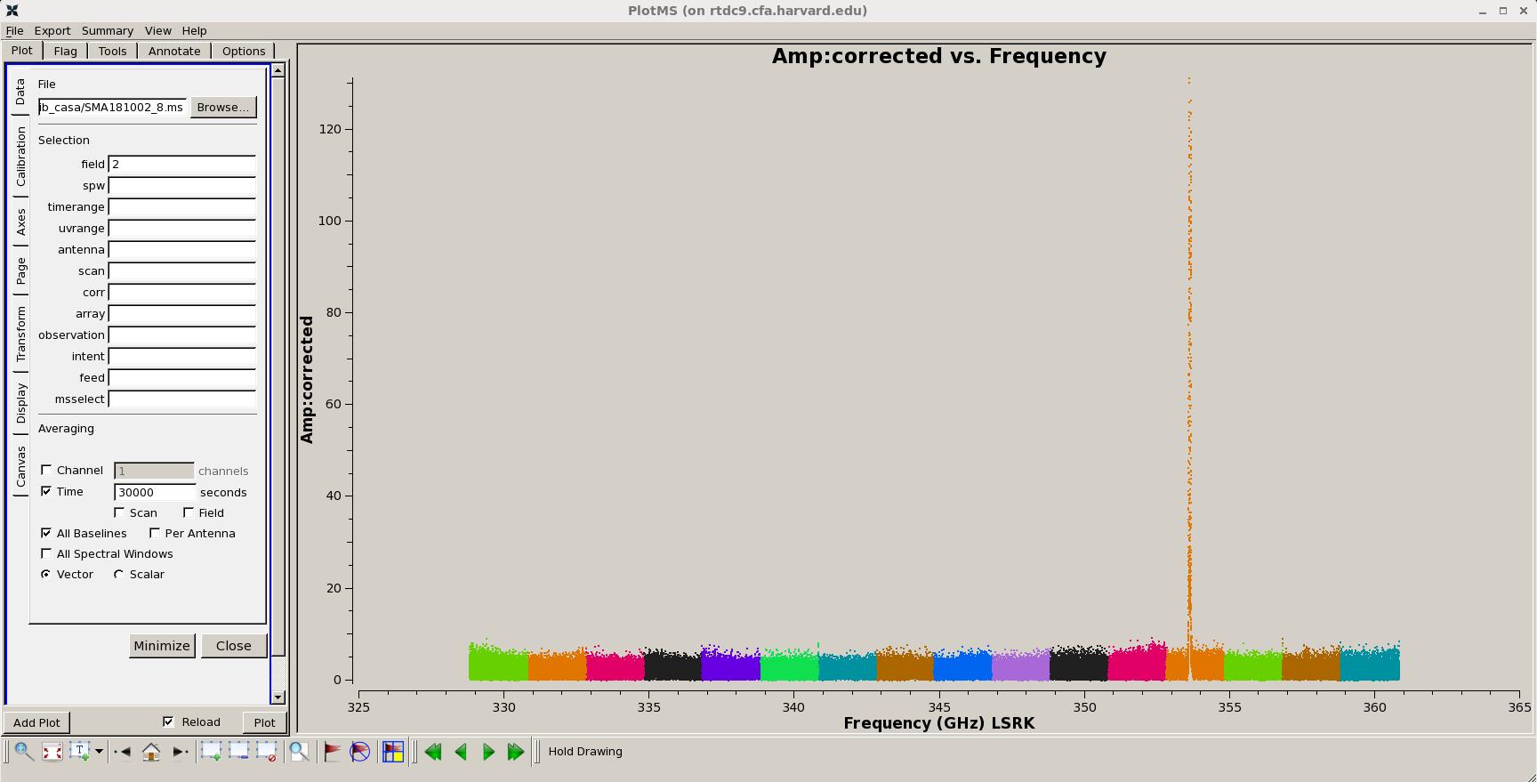
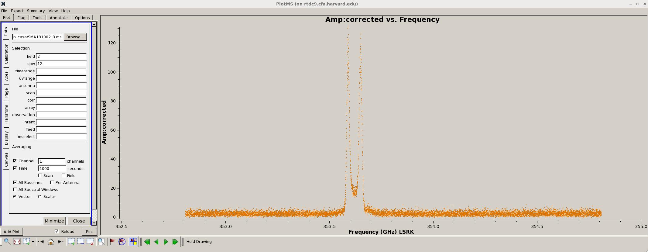
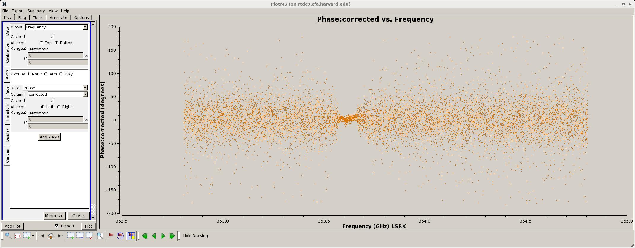 Fig. 19. Spetrum of the secondary target source (mwc349a). A hydrogen maser line (H26a) at
rest frequency 353.622795 GHz in spw 12 (orange) is prominent among all the 16 color-coded spectral windows (Top panel).
Middle panel show the well-know double-peaked spectral features. The phase of the H26a maser line is also plotted
(Bottom). Click the figure for enlargement.
Fig. 19. Spetrum of the secondary target source (mwc349a). A hydrogen maser line (H26a) at
rest frequency 353.622795 GHz in spw 12 (orange) is prominent among all the 16 color-coded spectral windows (Top panel).
Middle panel show the well-know double-peaked spectral features. The phase of the H26a maser line is also plotted
(Bottom). Click the figure for enlargement.
- Plot UV structure -
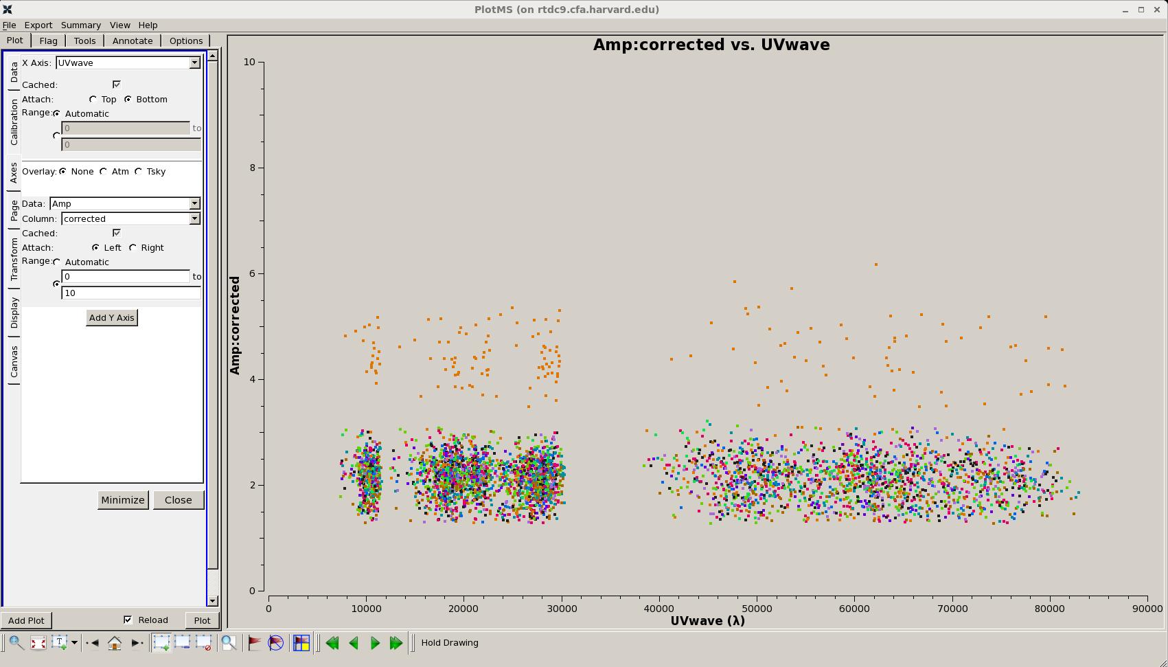 Fig. 20. UV structure of the econdary target source (mwc349a). Click the figure for enlargement.
T1(CKVul) -
- Plot spectra -

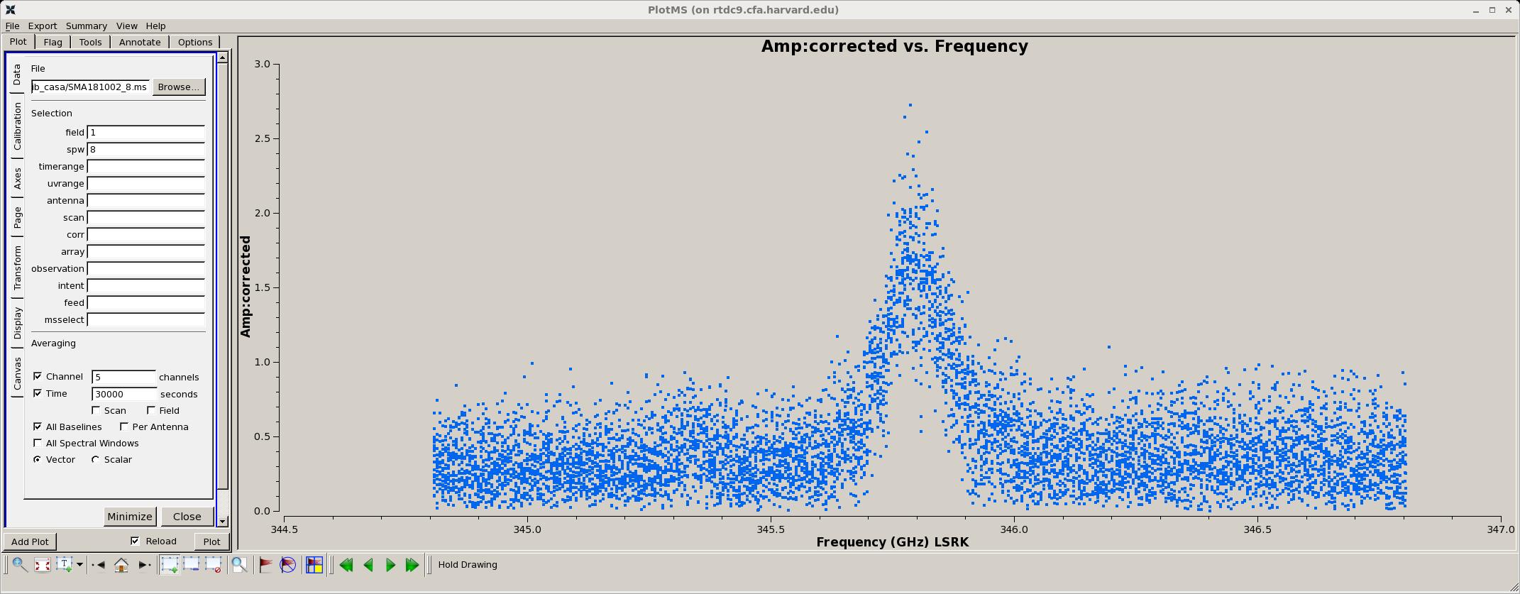

 Fig. 21. Spectrum of the primary target source (CKVul). There are three possible
spectral features are detected: spw8 (blue), the line peaked at 345.8 GHz;
spw3 (green), the line peaked at 330.6 GHz; and a weak one in spw12 (orange), the line peaked 354.6 GHz.
The three individual spw lines are shown followed the full (16) spw plot.
Click the figure for enlargement. The three line features are identified as
CO(3-2), 13CO(3-2) and HCN(4-3) at rest frequences of
345795.9899, 330587.9601, and 354505.4759 MHz, respectively.
____________________________
Note: The molecular lines were identified by the PI. The rest frequencies were from JPL Molecular Spectroscopy.
Fig. 21. Spectrum of the primary target source (CKVul). There are three possible
spectral features are detected: spw8 (blue), the line peaked at 345.8 GHz;
spw3 (green), the line peaked at 330.6 GHz; and a weak one in spw12 (orange), the line peaked 354.6 GHz.
The three individual spw lines are shown followed the full (16) spw plot.
Click the figure for enlargement. The three line features are identified as
CO(3-2), 13CO(3-2) and HCN(4-3) at rest frequences of
345795.9899, 330587.9601, and 354505.4759 MHz, respectively.
____________________________
Note: The molecular lines were identified by the PI. The rest frequencies were from JPL Molecular Spectroscopy.
- Plot UV structure -
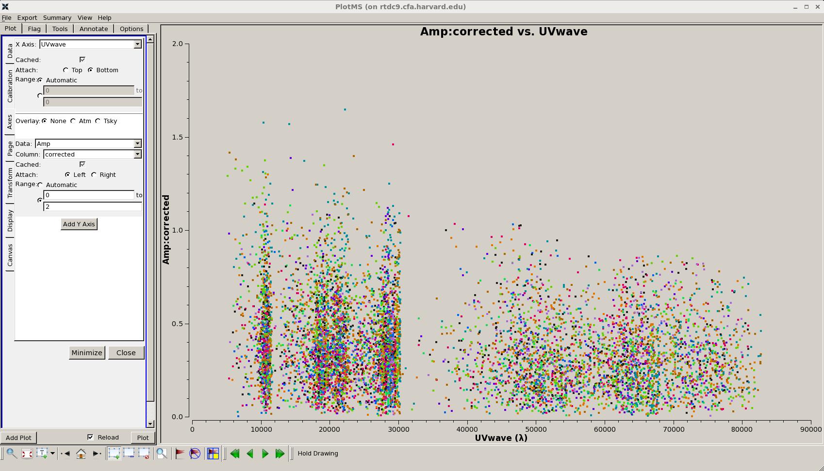 Fig. 22. UV structure of the primary target source (CKVul). Click the figure for enlargement.
Step 10: Split calibrated multi-source into single-source data -
CASA tasks:
     split
Usage of CASA-python-script module -
Step 11: Examine the calibrated data with imaging -
CASA tasks:
     clean (tclean)
     viewer
Usage of CASA-python-script module:
Image calibrators and the secondary target (continuum emission) -
Table 4: Images -
|
Examination of the calibrated data by making images
with Brigg's weight (R=2) or nature weight
|
|---|
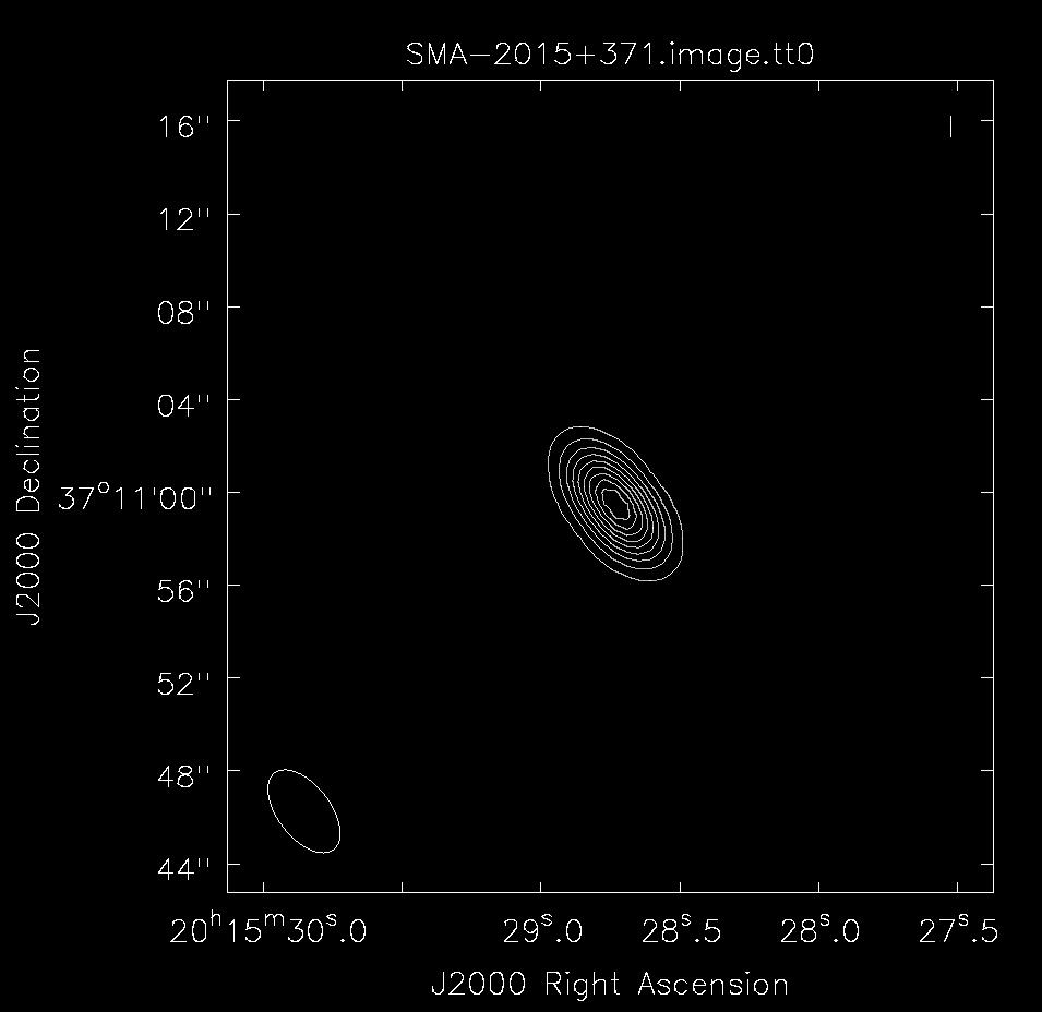
| 2015+371 (CG) |
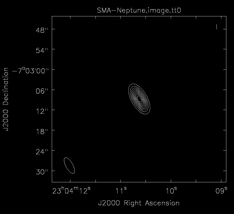
Neptune (FL) |
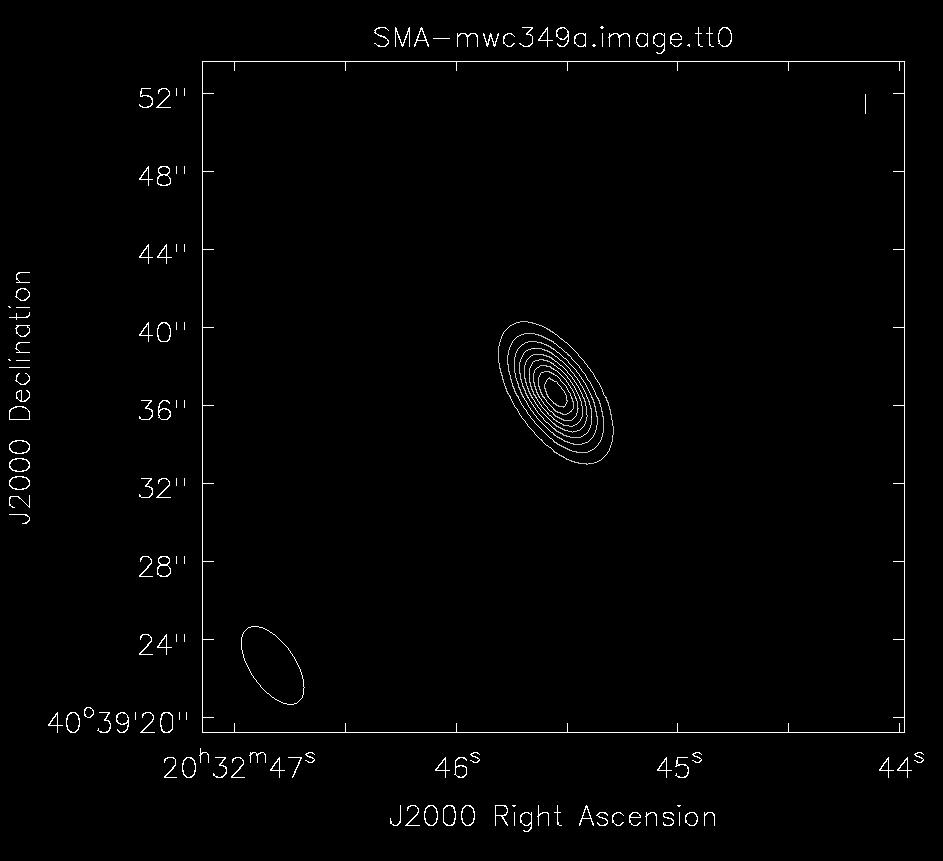
mwc349a (T2) |
3c84 (BP) |
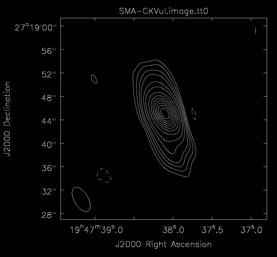
CKVul (T1) |
|
|
|

|
 |
|
Sp = 0.74 Jy/beam, rms = 0.002 Jy/beam, FWHM = 4.16"x2.26" (38 deg)
|
Sp = 20.1 Jy/beam, rms = 0.09 Jy/beam, FWHM = 5.26"x2.06" (28 deg)
|
Sp = 2.33 Jy/beam, rms = 0.003 Jy/beam, FWHM = 4.58"x2.29" (34 deg)
|
Sp=5.28 Jy/beam, rms = 0.005 Jy/beam, FWHM = 6.00"x2.16" (61 deg)
|
Sp=0.147 Jy/beam, rms = 1.1 mJy/beam,FWHM =4.62"x2.34" (30.7 deg) |
Note: Calibrators (2015+371, Neptune, mwc349a, 3c84) - contours are Sp x (-0.1, 0.1, 0.2, 0.3, 0.4,..., 0.8, 0.9).
Target (CKVul) - contours are Sp x (-0.04, 0.03, 0.05, 0.075, 0.1, 0.15, 0.2, 0.3 ..., 0.9).
Click an image for enlargement.
Imaging calibrated SWARM data -
Step 12: Image continuum data -
CASA tasks:
     plotms
     clean (tclean)
     viewer
Usage of CASA-python-script module:
Image CK Vul (T1) continuum emission -

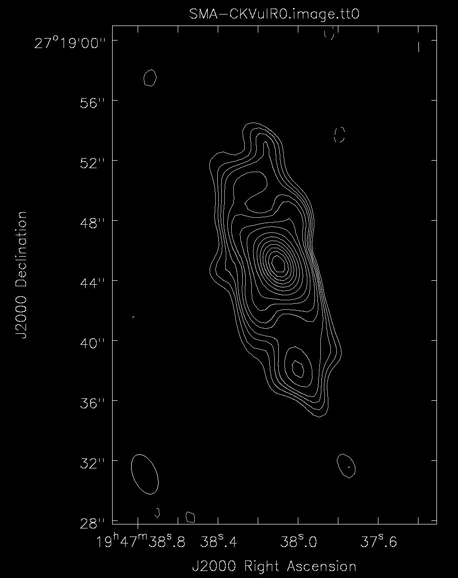
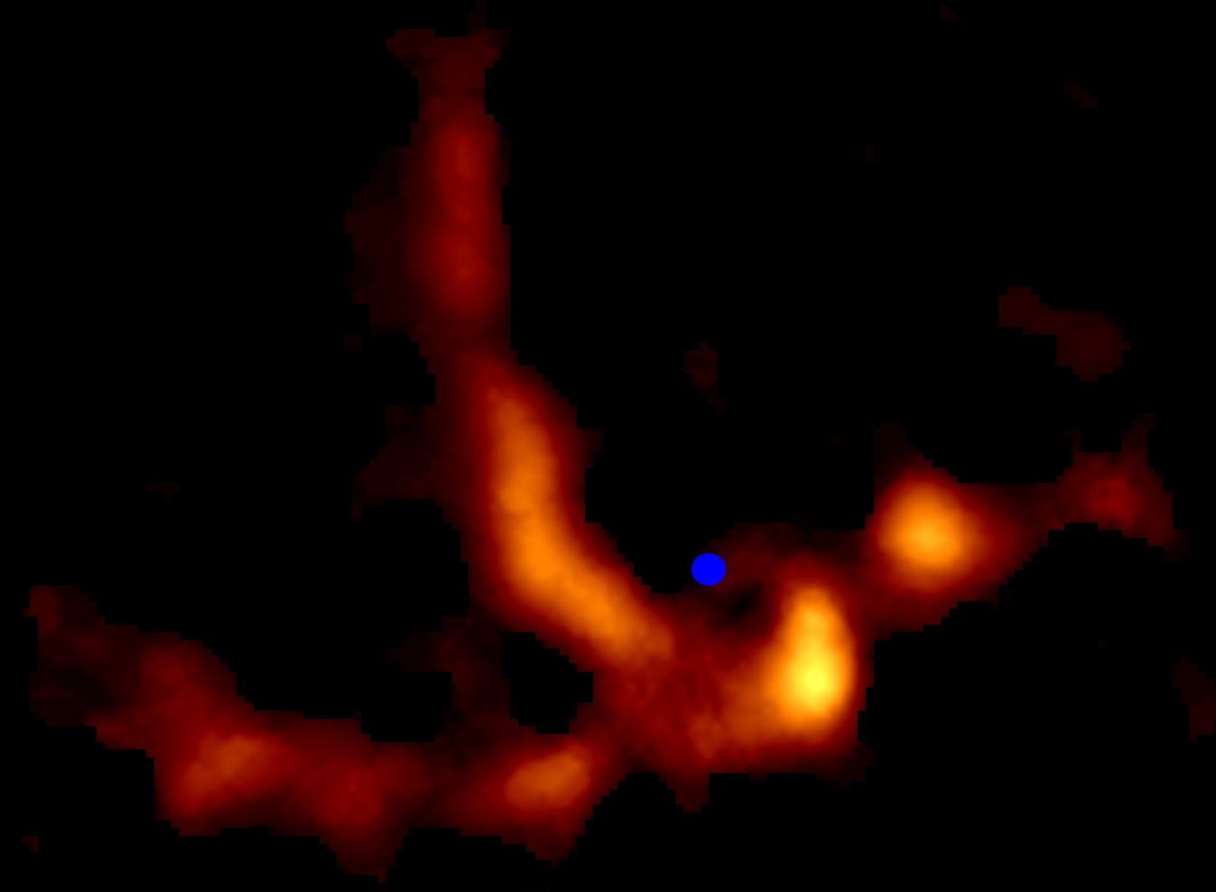
Fig. 23. SMA image of CKVul at 345 GHz with Brigg's weight (R=0).
Left: color version. Right: contour version. Contours = 92 mJy/Beam x (-0.03, 0.03, 0.04, 0.05, 0.06, 0.08, 0.1, 0.15, 0.2,
0.3, 0.4, 0.5, 0.6, 0.7, 0.8, 0.9),
rms = 0.9 mJy/beam. FWHM = 2.8"x 1.6" (23 deg).
Step 13: Identify spectral lines and construction image cubes -
CASA tasks:
     clean (tclean)
     viewer
     ...
Usage of CASA-python-script module -
To be done....
Step 14: Combine different array data -
CASA tasks:
     ...
Usage of CASA-python-script module:
180520_09:32:09 (extended array 2017B-S002), LO Freq: 341.1(B) 341.1(A). Sub-arcsec redolution (0.7"-0.8").
To be done....
Step 15: Convert CASA images to FITS -
CASA tasks:
     ...
Usage of CASA-python-script module:
|
| |
| |
|