![]()
![]()
![]()
![]()
![]()

![]()
![]()
![]()
|
|
|
|
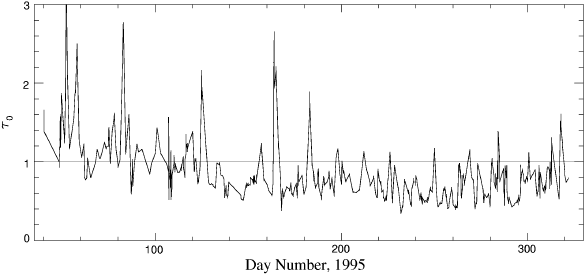
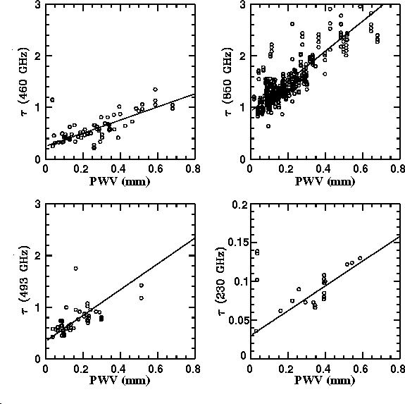
Opacity MeasurementsCARA experiments have directly measured both millimeter and submillimeter-wave atmospheric opacity at the South Pole using skydip techniques. Over 1100 skydip observations were made at 492 GHz (609 µm) with AST/RO during the 1995 observing season. Even though this frequency is near a strong oxygen line, the opacity was below 0.70 half of the time during the Austral winter and reached values as low as 0.34, better than ever measured at any ground-based site. The stability was also remarkably good: the opacity remained below 1.0 for weeks at a time. Skydip data at 225 GHz (1.33 mm) were obtained during 1993 by Richard Chamberlin and John Bally using a standard NRAO tipping radiometer similar to the ones used to measure the 225 GHz zenith opacities at Mauna Kea and the ALMA site at Chajnantor. The tight linear relation between 225 GHz skydip data and balloon sonde PWV measurements is discussed by Chamberlin and Bally (Int. J. IR and MM Waves, 16, 907).
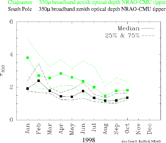
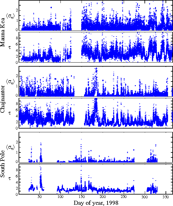
Of the three sites, South Pole consistently has the lowest water vapor and temperature but the highest pressure. This mixture makes the comparison between Pole and other sites more favorable at some wavelengths than at others. All three sites are excellent at millimeter-waves; the 225 GHz data for South Pole and Chajnantor are comparable because at that frequency the lower PWV at Pole is roughly balanced by the lower pressure at Chajnantor. Both are superior to Mauna Kea. From early 1998, the 350µm band has been continuously monitored at Mauna Kea, Chajnantor, and South Pole by identical tipper instruments developed by S. Radford of NRAO and J. Peterson of Carnegie-Mellon U. and CARA. These instruments measure a broad band that includes the center of the 350µm window as well as more opaque nearby wavelengths. Comparison of the opacity values measured by these instruments is tightly correlated with occasional narrow-band skydip measurements made within this band by the CSO and AST/RO; the narrow band opacity values are about a factor of two smaller than those output by the broadband instrument.
The South Pole PWV levels applicable 10%, 25%, 50%, and 75% of the time during winter have been used to compute values of atmospheric transmittance. For comparison, the transmittance for excellent conditions at Chajnantor is shown by the lowest dashed line in the figure. If three identical background-limited instruments operating in the 350µm window were placed at Pole, Chajnantor, and Mauna Kea to do identical observations over a long period of time, the observations at Pole would proceed 110 × faster than Mauna Kea and 4.5 × faster than Chajnantor.
|
|
Send mail to help@cfa.harvard.edu with
questions or comments about this web site.
|