 |
Abstract -
This reduction is used to test DopplerTrackerr_haystack patch using Todd Hunter's
SMA swarm data set 190314_11:50:03 of SMA project: 2019?-S??? with archived information:
PI                 - Todd Hunter
Target             - g358.93-0.03
RA (J2000)         - 17:43:10.05
Dec (J2000)        - −29:51:46.1
LO Freq (GHz)      - 298.4 (A), 210.9 (B) (A: 340 rx , B: 240 rx)
N-bsln             - 28(A), 28(B)
Angular resolution - 0.40"(B), 0.56"(B)
Time               - 208 min
Calibrators & targets -
T1:     G358.93-0.03
BP:     3c279
FL/BP2: Callisto
CG1:    1744-312
CG2:    1256-057
CG3:    1733-130
CG4:    1700-261
CG5:    1924-292
T2:     sgrb2n
T3:     ngc6334l
Following the steps of calibrations described in The example of CASA reduction of SMA data after pipeline the swarm data into CASA. SMA continuum image of G358.93-0.03 at 210 GHz
is constructed, in good agreement with ALMA 340 GHz image.
The 1σ rms noise of the SMA continuum image at 210 GHz (one receiver data with BW=16 GHz) is 0.4-0.5 mJy/beam in an angular
resolution of 0.9"x0.5".
_____________________________________
1The calibrator codes BP, CG, FL stand for bandpass, complex gain, and flux density. T stands for target.
Pipeline SWARM to CASA -
############################################
#define variables for swarm data reduction #
############################################
datain   = 'SMA190314_rx2'
inttime  = 9.68
dinttime = 20.
tinttime = 30.
qsecond  = 30.0
allspw   = '0~7'
allspw1  = '0~7:512~15871'
allspw2  = '0~7:1024~15359'
blckspw1 = '0~3:1024~15359'
blckspw2 = '4~7:1024~15359'
quadspw  = '0,2,4,6'
nchspw   = 16384
nchnew   =  1792
width0   =    1
width1   =    2
width2   =    4
width3   =    8
width4   =   16
width5   =   32
width6   =   64
width7   =  128
avgchan0 =   '1'
avgchan1 =   '2'
avgchan2 =   '4'
avgchan3 =   '8'
avgchan4 =  '16'
avgchan5 =  '32'
avgchan6 =  '64'
avgchan7 = '128'
#############################################
#user's setup below -                       #
#############################################
#
# Note for import data -
# the input measurementSet must be created via the swarm2casa path
#
#prefix of swarm measurementSet -
datain   = 'SMA190314_rx2'
#full name of swarm measurementSet -
datainms = 'SMA190314_rx2.ms'
#number of channels to average -
bw       = width3
#define source code -
BP =  '0'  #bandpass calibrator
BP2 = '1'  #optional bandpass calibrator
FL  = '1'  #flux density scale calibrator
CG  = '2,3,5'#complex gain calibrators
CG1 = '2'  #optional complex gain calibrator
CG2 = '3'  #optional complex gain calibrator
T1  = '4'  #primary target
CG3 = '5'  #optional complex gain calibrator
T2  = '6'  #secondary target
T3  = '7'  #secondary target
#define source name -
BPname  = '3c279'
BP2name = 'Callisto'
FLname  = 'Callisto'
CG1name = '1733-130'
CG2name = '1700-261'
CG3name = '1744-312'
CGname  = '1733-130, 1700-261, 1744-312'
T1name  = 'G358.93-0.03'
T2name  = 'sgrb2n'
T3name  = 'ngc6334l'
#define reference antenna -
rant = '5'
#
Step 1: Prepare for calibration-
CASA tasks:
     listobs
     plotants
     split  (not used)
Usage of CASA-python-script module -
Listobs output -
Table 1: Source/Field information -
| Source (Field) information reported from CASA listobs |
|---|
| ID |
Code# |
Name |
RA |
Decl |
Epoch |
SrcId |
nRows |
|
0 | BP | 3c279 | 12:56:11.165085 | −05:47:21.52451 | J2000 | 0 | 84672 | |
1 | FL/BP2 | Callisto | 17:30:06.907654 | −22.37.37.71790 | J2000 | 1 | 34720 | |
2 | CG1 | 1733-130 | 17:33:02.702637 | −13.04.49.54811 | J2000 | 2 | 46144 | |
3 | CG2/CG | 1700-261 | 17:00:53.153229 | −26.10.51.72272 | J2000 | 3 | 99232 | |
4 | T1 | G358.93-0.03 | 17:43:10.047455 | −29.51.46.13022 | J2000 | 4 | 289632 | |
5 | CG3/CG | 1744-312 | 17:44:23.580322 | −31.16.35.98618 | J2000 | 5 | 47488 | |
6 | T2 | sgrb2n | 17:47:19.876556 | −28.22.18.38196 | J2000 | 6 | 7168 | |
7 | T3 | ngc6334l | 17:20:53.423309 | −35.46.57.89703 | J2000 | 7 | 8288 |
________________
*Check listobs_log for the issue of source ID and spw mix-up
#Note for Code:
BP - bandpass
CG - complex gain
T1 - Target source
T2 - Secondary target source for examing calibration
T3 - Secondary target source for examing calibration
FL - Flux density scale calibrator
$ BP2 = FL - Callisto is an option to be used to solve for bandpass
Table 2: Correlator/Frequency configuration, original -
|
Spectral Windows: (16 unique spectral windows and 1 unique polarization setups) |
|---|
| SpwID |
Name |
#Chans |
Frame |
Ch0(MHz) |
ChanWid(kHz) |
TotBW(kHz) |
CtrFreq(MHz) |
Corrs |
|
0 | none | 16384 | LSRK | 207034.258 | -139.648 | 2288000.0 | 205890.3274 | XX | |
1 | none | 16384 | LSRK | 202735.106 | 139.648 | 2288000.0 | 203879.0364 | XX | |
2 | none | 16384 | LSRK | 203034.787 | -139.648 | 2288000.0 | 201890.8570 | XX | |
3 | none | 16384 | LSRK | 198735.635 | 139.648 | 2288000.0 | 199879.5656 | XX | |
4 | none | 16384 | LSRK | 214733.518 | 139.648 | 2288000.0 | 215877.4487 | XX | |
5 | none | 16384 | LSRK | 219032.670 | -139.648 | 2288000.0 | 217888.7400 | XX | |
6 | none | 16384 | LSRK | 218732.989 | 139.648 | 2288000.0 | 219876.9191 | XX | |
7 | none | 16384 | LSRK | 223032.139 | -139.648 | 2288000.0 | 221888.2091 | XX |
- Plot antenna array -
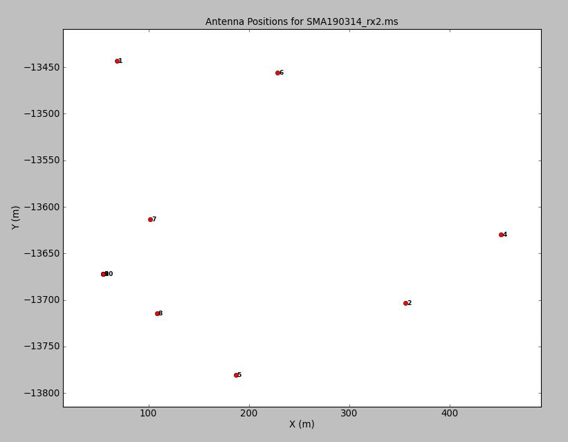 Fig. 1: Antenna array. Click the figure for enlargement.
Split & bin data -
Listobs output (binned data) -@
_____________________________________
@Note: the original spectral data are binned with
bw = width3, or vector-averaging 8 channels to produce a new channel width of 1.117188 MHz,
which provides an adequate velocity resolution (1 km/s) for this project.
Step 2: Inspecting and editing data -
CASA tasks:
plotms
Usage of CASA-python-script module -
- Plot uv-coverage -
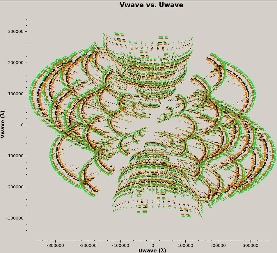 Fig. 2: uv-coverage (spw 0,4,8,12) (all fields). Click the figure for enlargement.
- Plot elevation coverage -
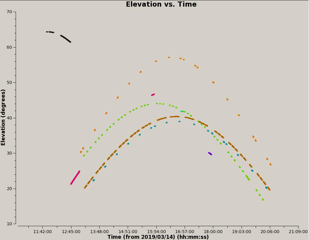 Fig. 3: Elevation coverage including all field (0~5).
Black: 0 BP 3c273;
Red: 1 FL Collisto;
Orange: 2 CG1 1733-130;
Green: 3 CG2 1700-261;
Brown: 4 T1 G358.93-0.03;
Blue: 5 T2 sgrb2n;
Purple: 6 T3 ngc6334l.
Click the figure for enlargement.
Fig. 3: Elevation coverage including all field (0~5).
Black: 0 BP 3c273;
Red: 1 FL Collisto;
Orange: 2 CG1 1733-130;
Green: 3 CG2 1700-261;
Brown: 4 T1 G358.93-0.03;
Blue: 5 T2 sgrb2n;
Purple: 6 T3 ngc6334l.
Click the figure for enlargement.
- Plot fringe amplitude vs time -
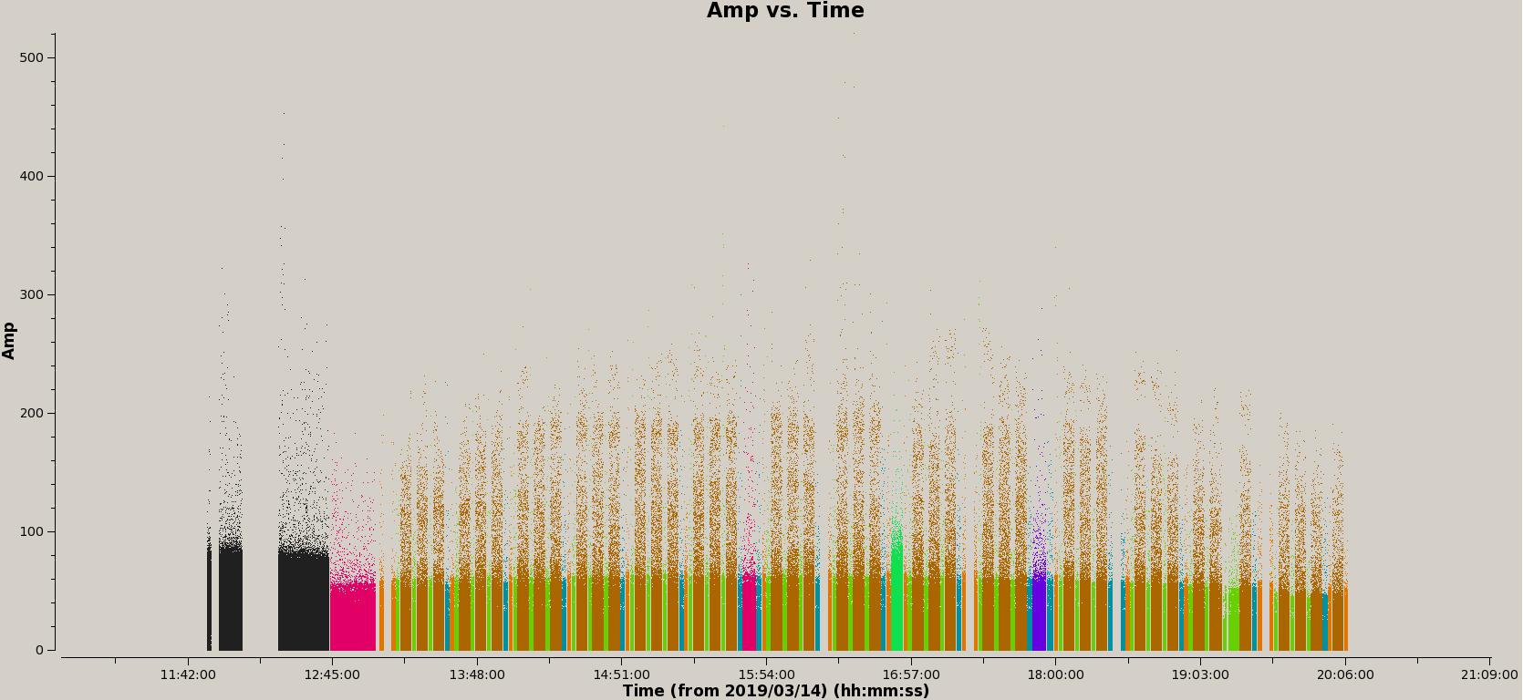 Fig. 4: Fringe amplitude vs time after flagging a few high-amplitude spikes in the inspect&editing cycle (pre-calibration).
Black: 0 BP 3c273;
Red: 1 FL Collisto;
Orange: 2 CG1 1733-130;
Green: 3 CG2 1700-261;
Brown: 4 T1 G358.93-0.03;
Blue: 5 T2 sgrb2n;
Purple: 6 T3 ngc6334l.
Click the figure for enlargement.
Fig. 4: Fringe amplitude vs time after flagging a few high-amplitude spikes in the inspect&editing cycle (pre-calibration).
Black: 0 BP 3c273;
Red: 1 FL Collisto;
Orange: 2 CG1 1733-130;
Green: 3 CG2 1700-261;
Brown: 4 T1 G358.93-0.03;
Blue: 5 T2 sgrb2n;
Purple: 6 T3 ngc6334l.
Click the figure for enlargement.
Step 3: Set flux density scale -
CASA tasks:
setjy
Usage of CASA-python-script module -
Note: FL is Neptune that is used to set the flux-density scale with the model standard:
Butler-JPL-Horizons 2012
Setjy output -
Table 3: Results of setjy -
|
FL is Callisto that is used to set the flux-density scale with the model standard:
Butler-JPL-Horizons 2012 |
|---|
| Reference source |
Specral window |
Flux density |
Frequency |
|
Callisto: | spw0 | Flux:[I=4.2679,Q=0.0,U=0.0,V=0.0] +/- [I=0.0,Q=0.0,U=0.0,V=0.0] Jy | @ 207.03GHz | |
Callisto: | spw1 | Flux:[I=4.0877,Q=0.0,U=0.0,V=0.0] +/- [I=0.0,Q=0.0,U=0.0,V=0.0] Jy | @ 202.74GHz | |
Callisto: | spw2 | Flux:[I=4.1002,Q=0.0,U=0.0,V=0.0] +/- [I=0.0,Q=0.0,U=0.0,V=0.0] Jy | @ 203.03GHz | |
Callisto: | spw3 | Flux:[I=3.9241,Q=0.0,U=0.0,V=0.0] +/- [I=0.0,Q=0.0,U=0.0,V=0.0] Jy | @ 198.74GHz | |
Callisto: | spw4 | Flux:[I=4.6005,Q=0.0,U=0.0,V=0.0] +/- [I=0.0,Q=0.0,U=0.0,V=0.0] Jy | @ 214.73GHz | |
Callisto: | spw5 | Flux:[I=4.7912,Q=0.0,U=0.0,V=0.0] +/- [I=0.0,Q=0.0,U=0.0,V=0.0] Jy | @ 219.03GHz | |
Callisto: | spw6 | Flux:[I=4.7778,Q=0.0,U=0.0,V=0.0] +/- [I=0.0,Q=0.0,U=0.0,V=0.0] Jy | @ 218.73GHz | |
Callisto: | spw7 | Flux:[I=4.9717,Q=0.0,U=0.0,V=0.0] +/- [I=0.0,Q=0.0,U=0.0,V=0.0] Jy | @ 223.03GHz |
Step 4: Solve for delay & bandpass -
CASA tasks:
     plotms
     gaincal
     bandpass
     plotcal
Usage of CASA-python-script module -
Note: using the BP (3c279) to solve for delay.
- Plot delay corrections -
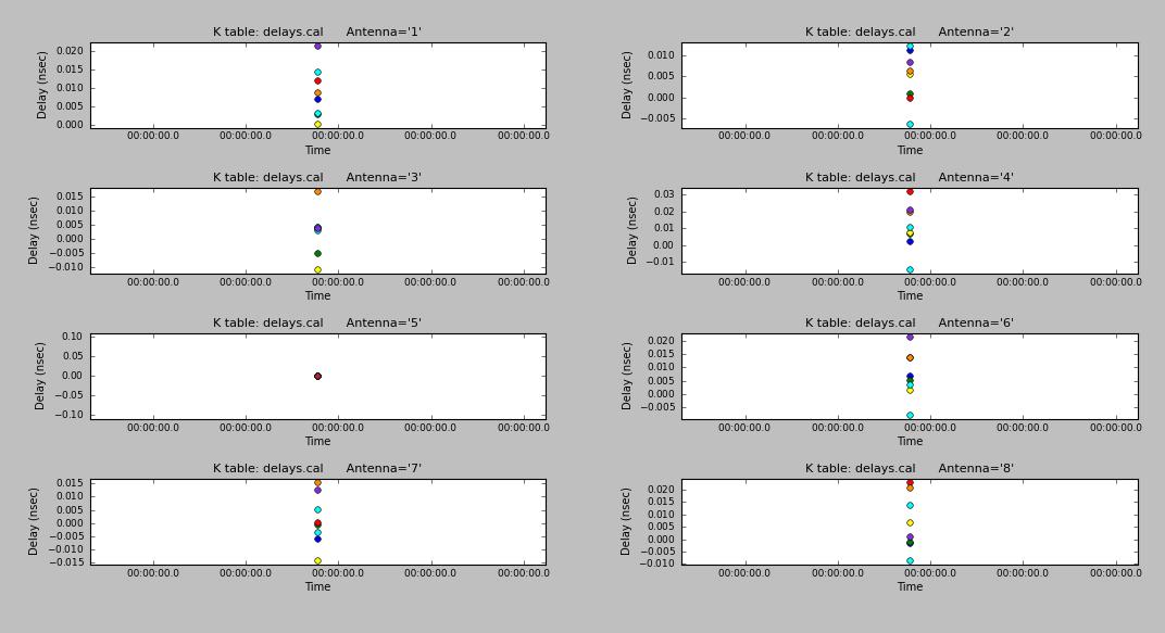 Fig. 5: Antenna-based delay as function of time. The remaining delay shows a typical value of a few tens pico seconds,
quite small. Click the figure for enlargement.
Fig. 5: Antenna-based delay as function of time. The remaining delay shows a typical value of a few tens pico seconds,
quite small. Click the figure for enlargement.
Note: two options of solving for bandpass
- Option 1: 3c279 as defined early as a variable BP -
- Option 2: Callisto is weaker.
(BP2) -
- Plot bandpass phase correction -

Fig. 6: Antenna-based phase soultions as function of time solvd for BP, which needs to be applied to the data while
solving for bandpass. Click the figure for enlargement.
OPTION 1 -
- Plot bandpass amplitude-
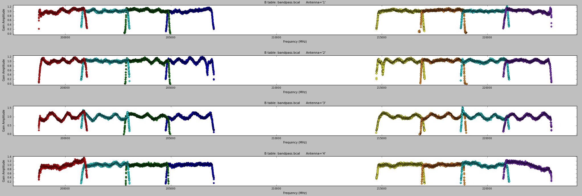
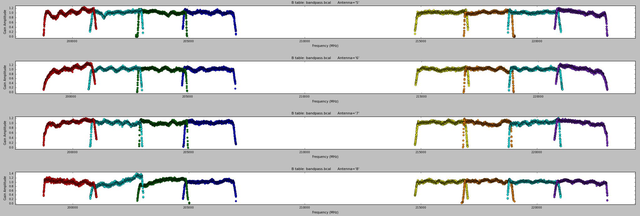 Fig. 7: Antenna-based bandpass solutions (amplitude) for option 1 (BP=3c84), solved with averaging every 16 channels. Top panel for antennas 1~4; bottom panel for
antenna 5~8. Click the figure for enlargement.
Fig. 7: Antenna-based bandpass solutions (amplitude) for option 1 (BP=3c84), solved with averaging every 16 channels. Top panel for antennas 1~4; bottom panel for
antenna 5~8. Click the figure for enlargement.
- Plot bandpass phase-
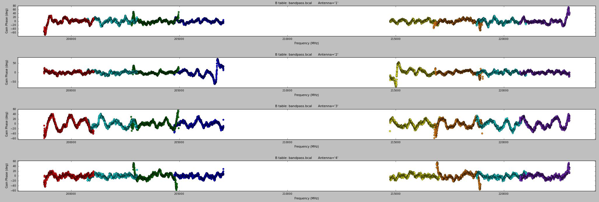
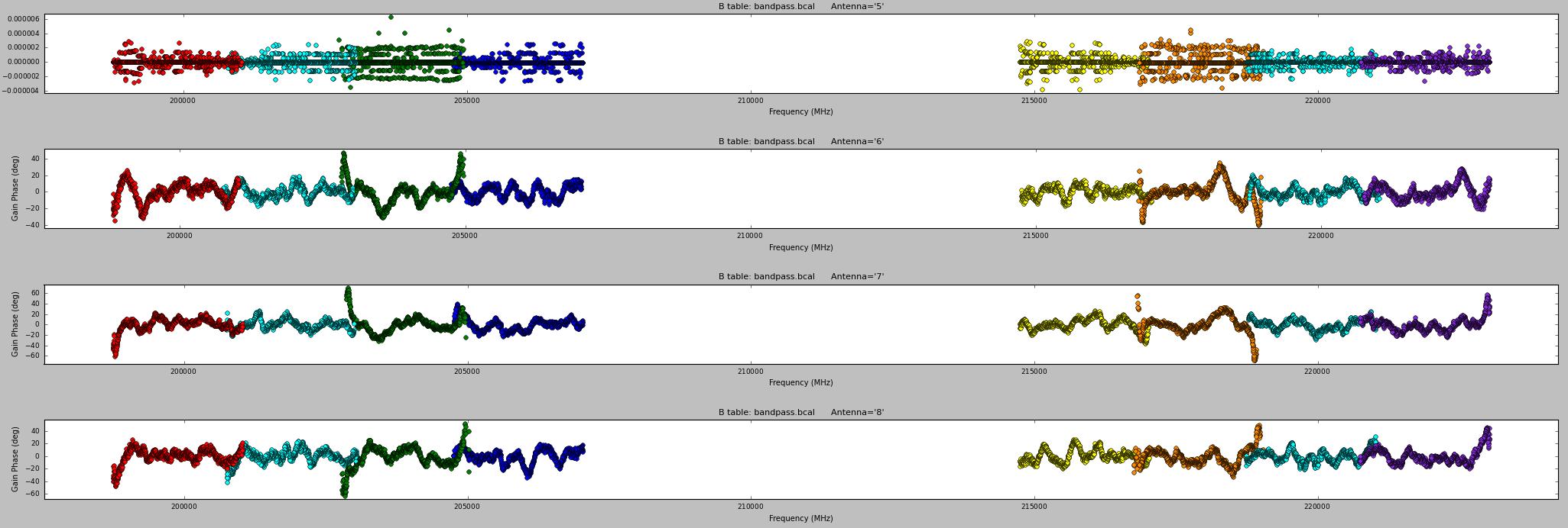 Fig. 8: Antenna-based bandpass solutions (phase) for option 1 (BP=3c84), solved with averaging every 16 channels. Top panel for antennas 1~4; bottom panel for
antenna 5~8. Click the figure for enlargement.
Fig. 8: Antenna-based bandpass solutions (phase) for option 1 (BP=3c84), solved with averaging every 16 channels. Top panel for antennas 1~4; bottom panel for
antenna 5~8. Click the figure for enlargement.
OPTION 2 -
- Plot bandpass amplitude-
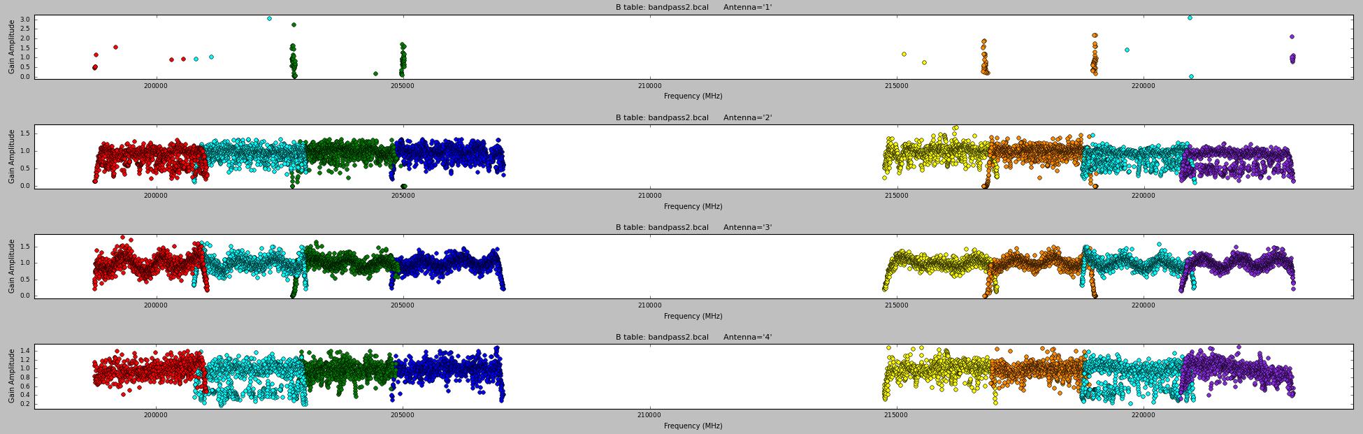
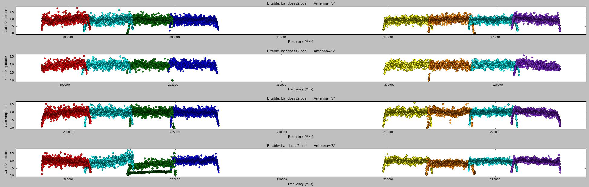 Fig. 9: Antenna-based bandpass solutions (amplitude) for option 2 (BP2=Neptune), solved with each channel. Top panel for antennas 1~4; bottom panel for
antenna 5~8. Click the figure for enlargement.
Fig. 9: Antenna-based bandpass solutions (amplitude) for option 2 (BP2=Neptune), solved with each channel. Top panel for antennas 1~4; bottom panel for
antenna 5~8. Click the figure for enlargement.
- Plot bandpass phase-
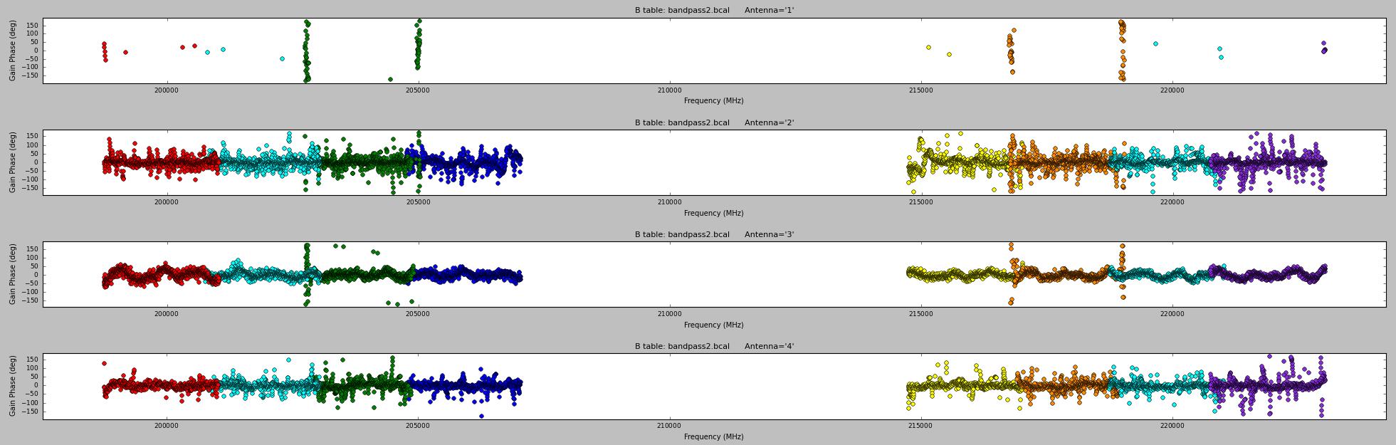
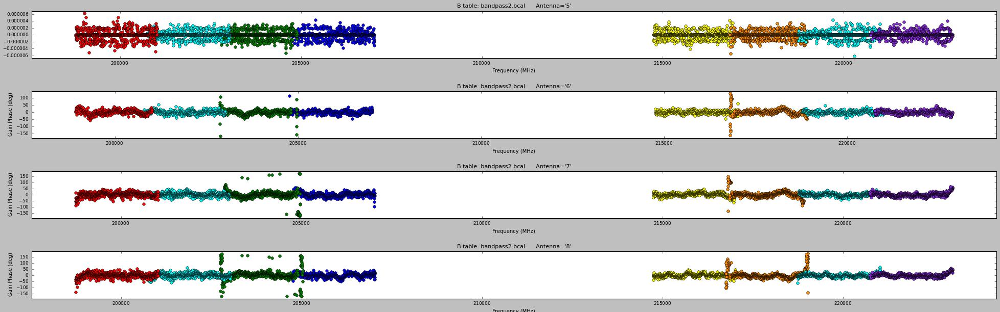 Fig. 10: Antenna-based bandpass solutions (phase) for option 1 (BP2=Neptune), solved with each channel. Top panel for antennas 1~4; bottom panel for
antenna 5~8. Click the figure for enlargement.
Fig. 10: Antenna-based bandpass solutions (phase) for option 1 (BP2=Neptune), solved with each channel. Top panel for antennas 1~4; bottom panel for
antenna 5~8. Click the figure for enlargement.
Step 5: Apply the delay and bandpass solution to the BP, CG, FL data -
CASA tasks:
     applycal
     plotms
Usage of CASA-python-script module -
Note: edting the data before next step
Step 6: Solve for complex gains -
CASA tasks:
     gaincal
     plotcal
Usage of CASA-python-script module:
Note: solving for complex gains for the calibrators FL, BP and CG prior to bootstrape the flux-density scale
- Plot phase solutions in integration-
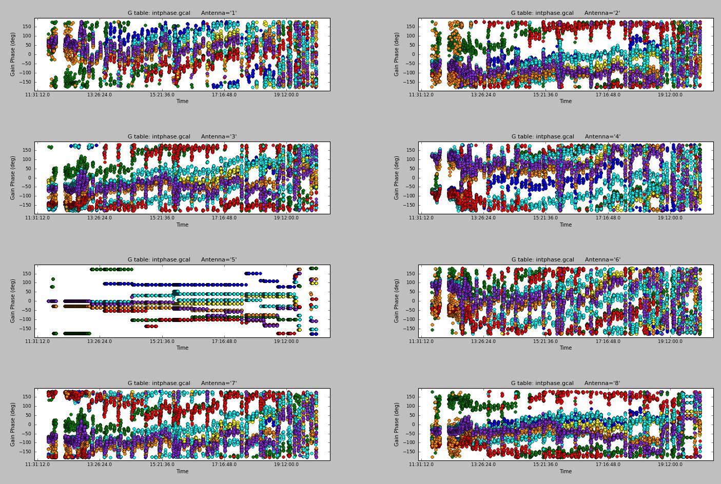 Fig. 11. Antenna-based phase solutions (integration) for the calibrators FL, BP and CG.
Click the figure for enlargement.
Fig. 11. Antenna-based phase solutions (integration) for the calibrators FL, BP and CG.
Click the figure for enlargement.
- Plot phase solutions in scan-
 Fig. 12. Antenna-based phase solutions (scan) for the calibrators FL, BP and CG.
Click the figure for enlargement.
Fig. 12. Antenna-based phase solutions (scan) for the calibrators FL, BP and CG.
Click the figure for enlargement.
Step 7: Bootstrap flux-density scale from a reference source (FLname: Neptune) -
CASA tasks:
     fluxscale
Usage of CASA-python-script module:
Note: Report from CASA bootstraping
Table 4: A summary of flux density bootstraping -
|
Statistics of flux-density from the 16 spws |
|---|
| Calibrators |
Flux density and 1 σ uncertainty (Jy) |
Spectral index and 1 σ uncertainty |
Frequency(GHz) |
|
3c279 | 8.07928 +/- 0.617503 | −0.542301 +/- 1.53944 | 210.73 | |
1733-130 | 1.62645 +/- 0.00275459 | −0.602464 +/- 0.0435007 | 210.73 | |
1700-261 | 1.12312 +/- 0.00309053 | −0.310968 +/- 0.0722647 | 210.73 | |
1744-312 | 0.277765 +/- 0.00452225 | −0.673763 +/- 0.434288 | 210.73 |
Step 8: Apply calibration solutions to the data -
CASA tasks:
     applycal
Usage of CASA-python-script module:
Note: apply the calibrations to all the calibrators and target sources interested:
- 3c279 (BP),
- 1733-130 (CG1),
- 1700-261 (CG2),
- 1744-312 (CG3),
- Callisto (FL),
- G358.93-0.03 (T1), primary target
- sgrb2n (T2), secondary target
Step 9: Examine and edit calibrated data -
CASA tasks:
     plotms
Usage of CASA-python-script module:
Plot vis structure -
- BP(3c279) -
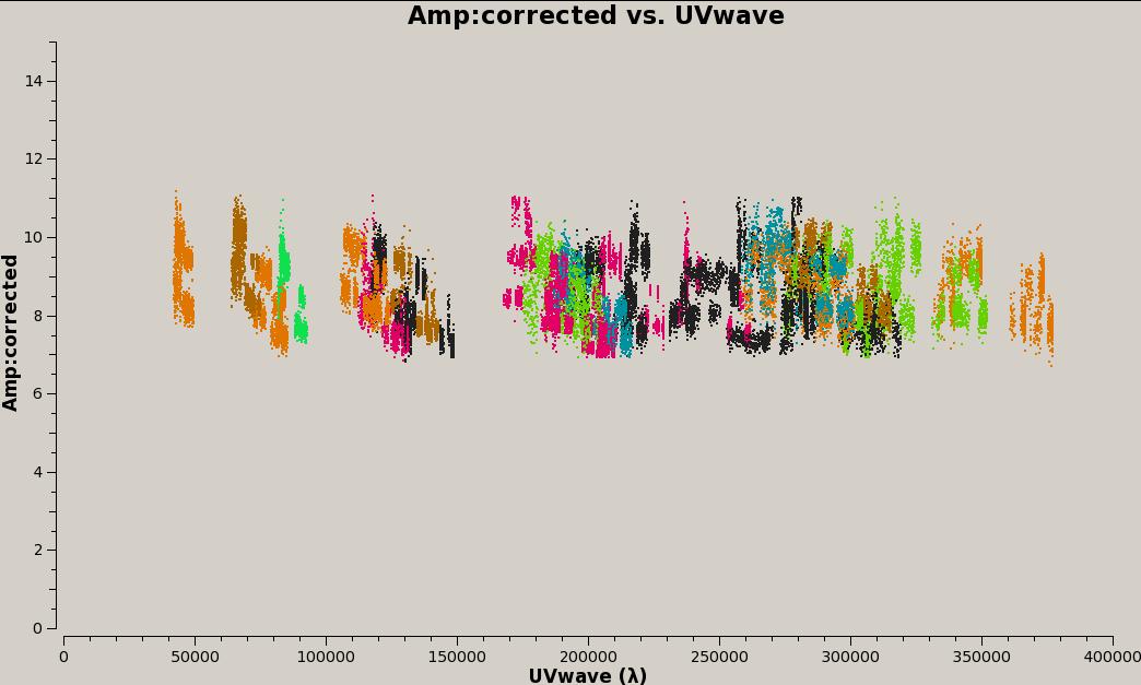
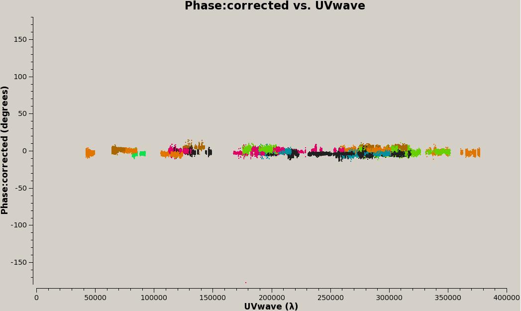 Fig. 13 Vis structure of bandpass calibrator (3c279). Top: amplitude. Bottom: phase.
Click the figure for enlargement.
Fig. 13 Vis structure of bandpass calibrator (3c279). Top: amplitude. Bottom: phase.
Click the figure for enlargement.
- FL(Callisto) -
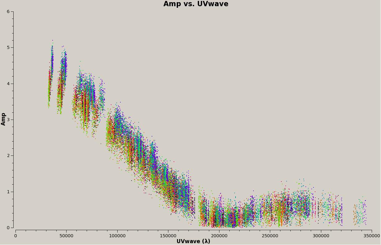
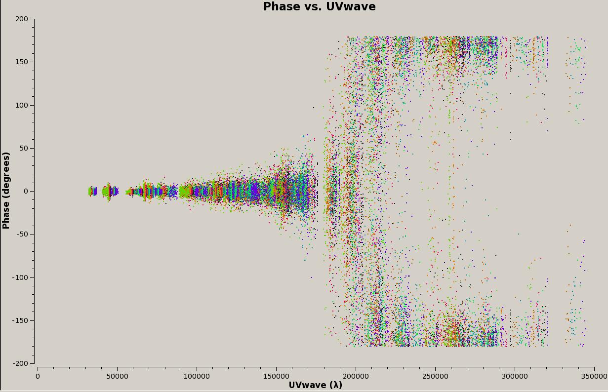 Fig. 14. UV structure of the Flux-density calibrator (Callisto),
amplitude (top) and phase (bottom). Click the figure for enlargement.
Fig. 14. UV structure of the Flux-density calibrator (Callisto),
amplitude (top) and phase (bottom). Click the figure for enlargement.
- CG1(1733-130) -
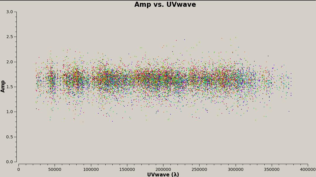
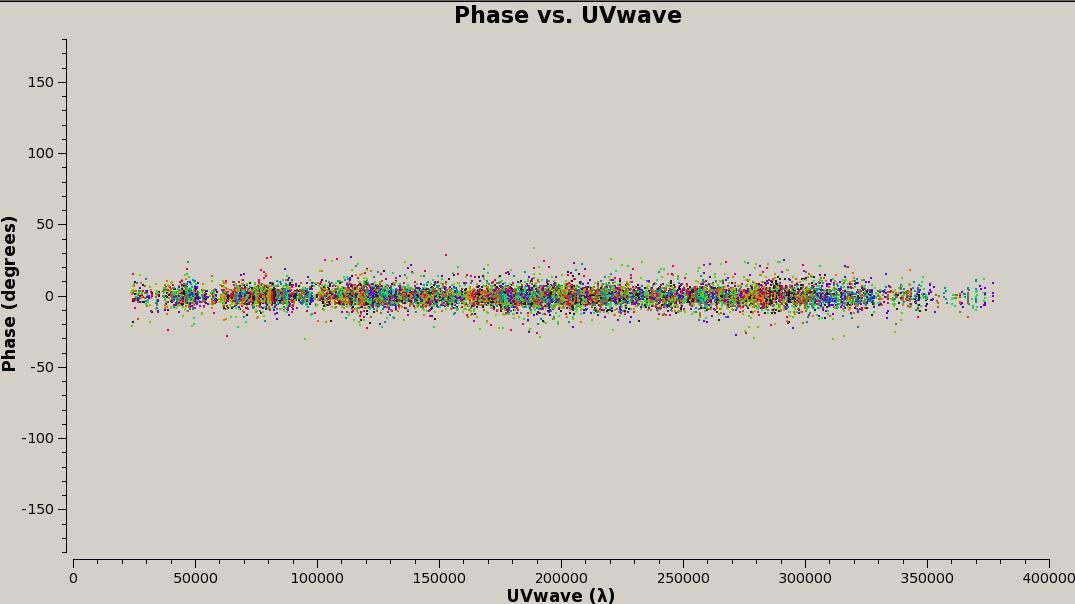 Fig. 15. Spetrum of the Complex gain calibrator1 (1733-130 (NRAO530)),
amplitude (top) and phase (bottom). Click the figure for enlargement.
Fig. 15. Spetrum of the Complex gain calibrator1 (1733-130 (NRAO530)),
amplitude (top) and phase (bottom). Click the figure for enlargement.
- CG2(1700-261) -
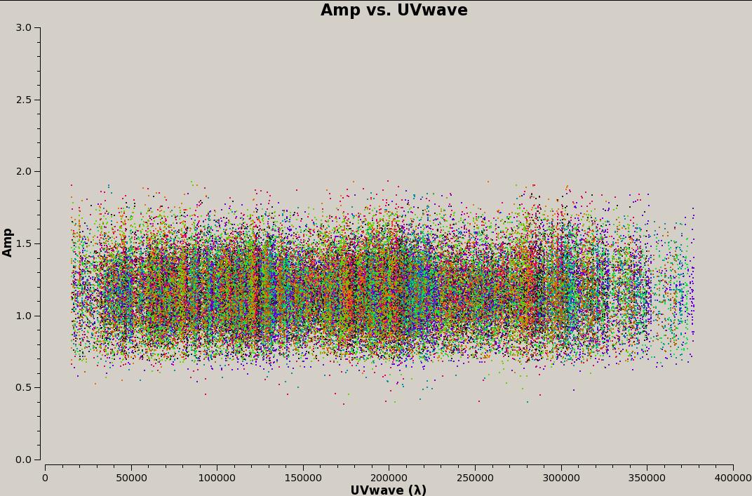
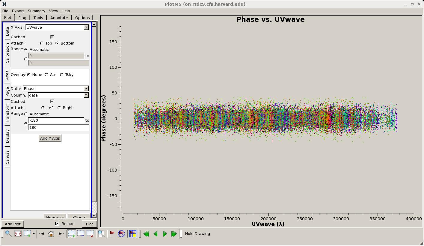 Fig. 16. UV structure of the Complex gain calibrator2 (1700-321 ( the main gain calinrator)),
amplitude (top) and phase (bottom). Click the figure for enlargement.
Fig. 16. UV structure of the Complex gain calibrator2 (1700-321 ( the main gain calinrator)),
amplitude (top) and phase (bottom). Click the figure for enlargement.
- CG3(1744-312) -

 Fig. 17. UV structure of calibrator3 (1744-312) after applying the corrections,
amplitude (top) and phase(bottom).
Click the figure for enlargement.
Fig. 17. UV structure of calibrator3 (1744-312) after applying the corrections,
amplitude (top) and phase(bottom).
Click the figure for enlargement.
- T1(G358.93-0.03) -
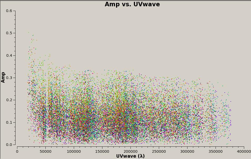
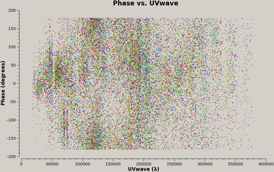 Fig. 18. UV structure of the target source (G358.93-0.03). Click the figure for enlargement.
Step 10: Split calibrated multi-source into single-source data for continuum and CH2OH lines -
CASA tasks:
     split
Usage of CASA-python-script module -
Step 11: Examine the calibrated data with imaging -
CASA tasks:
     clean (tclean)
     viewer
Usage of CASA-python-script module:
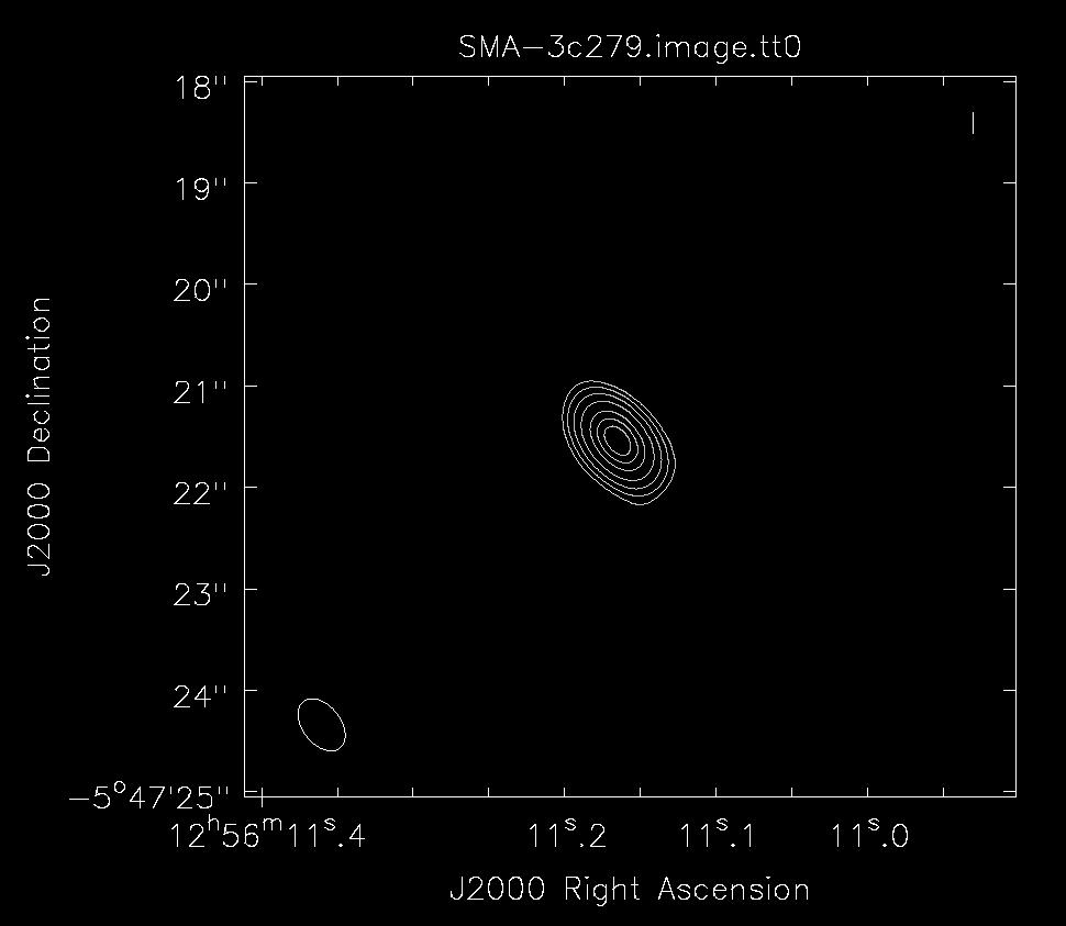
Image calibrators and the secondary target (continuum emission) -
Table 4: Images -
|
Examination of the calibrated data by making images
with Brigg's weight (R=2) or nature weight
|
|---|
| 3c279 (BP) |
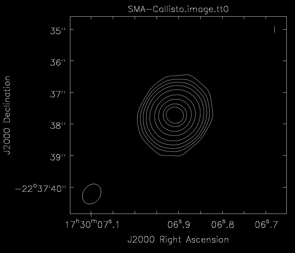
Callisto (FL) |
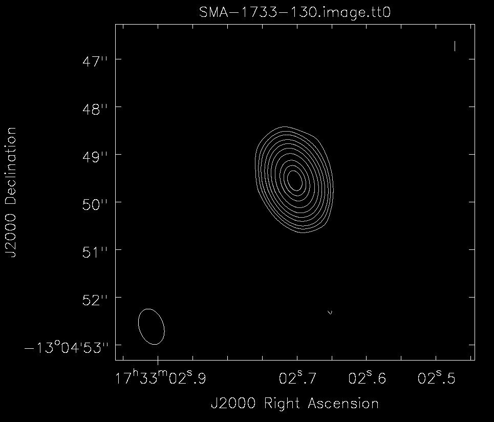
1733-130 (CG1) |
1700-261 (CG2) |
1744-312 (CG3) |
G358.93-0.03 (T1) |
|
|
|
|
|
|
|
Sp = 8.505 Jy/beam, rms = 20 mJy/beam, contours=Sp x (-0.025, 0.025, 0.05, 0.1, 0.2, 0.4, 0.6, 0.8)
|
Sp = 1.428 Jy/beam, rms = 2 mJy/beam, contours=Sp x (-0.01, 0.01, 0.025, 0.05, 0.1, 0.2, 0.4, 0.6, 0.8, 0.9)
|
Sp = 1.633 Jy/beam, rms = 0.8 mJy/beam, contours=Sp x (-0.002, 0.002, 0.005, 0.01, 0.025, 0.05, 0.1, 0.2, 0.4, 0.6, 0.8)
|
Sp=1.144 Jy/beam, rms = 0.5 mJy/beam, contours=Sp x (-0.002, 0.002, 0.005, 0.01, 0.025, 0.05, 0.1, 0.2, 0.4, 0.6, 0.8)
|
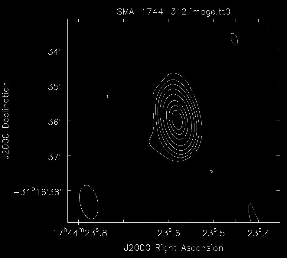
Sp=0.293 Jy/beam, rms = 1.0 mJy/beam, contours=Sp x (-0.01, 0.01, 0.025, 0.05, 0.1, 0.2, 0.4, 0.6, 0.8)
|
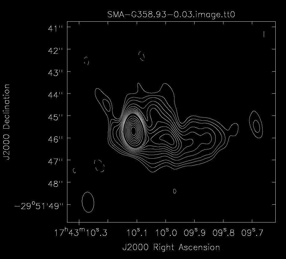
Sp=0.0897 Jy/beam, rms = 0.5 mJy/beam, contours=Sp x (-0.02, 0.02, 0.03, 0.04, 0.06, 0.08, 0.1, 0.12, 0.14, 0.16, 0.18,
0.2, 0.3, 0.4, 0.5, 0.6, 0.7, 0.8, 0.9) |
Note: The images are made with weight R=2; the synthesized beam is 0.9"x0.5".
Click an image for enlargement.
Imaging calibrated SWARM data -
Step 12: Image continuum data -
CASA tasks:
     plotms
     clean (tclean)
     viewer
Usage of CASA-python-script module:
- Image Callisto brightness distribution -
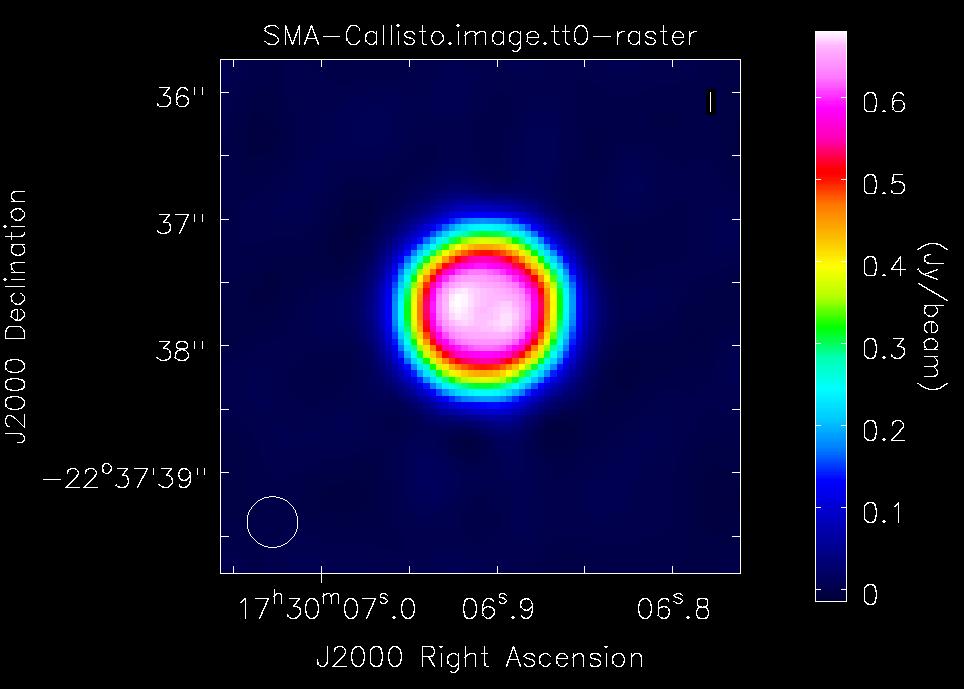 Fig. 19: Image of Callisto at 210.88 GHz by synthesizing 8 x 2GHz spws with weight R=-0.5. Sp=0.835 Jy/beam, St=5.174 Jy, rms =3.6 mJy/beam;
A circular beam with FWHM = 0.4" was used to convolve the clean components for the final image.
Fig. 19: Image of Callisto at 210.88 GHz by synthesizing 8 x 2GHz spws with weight R=-0.5. Sp=0.835 Jy/beam, St=5.174 Jy, rms =3.6 mJy/beam;
A circular beam with FWHM = 0.4" was used to convolve the clean components for the final image.
- Image G358.93-0.03 (T1) continuum emission -
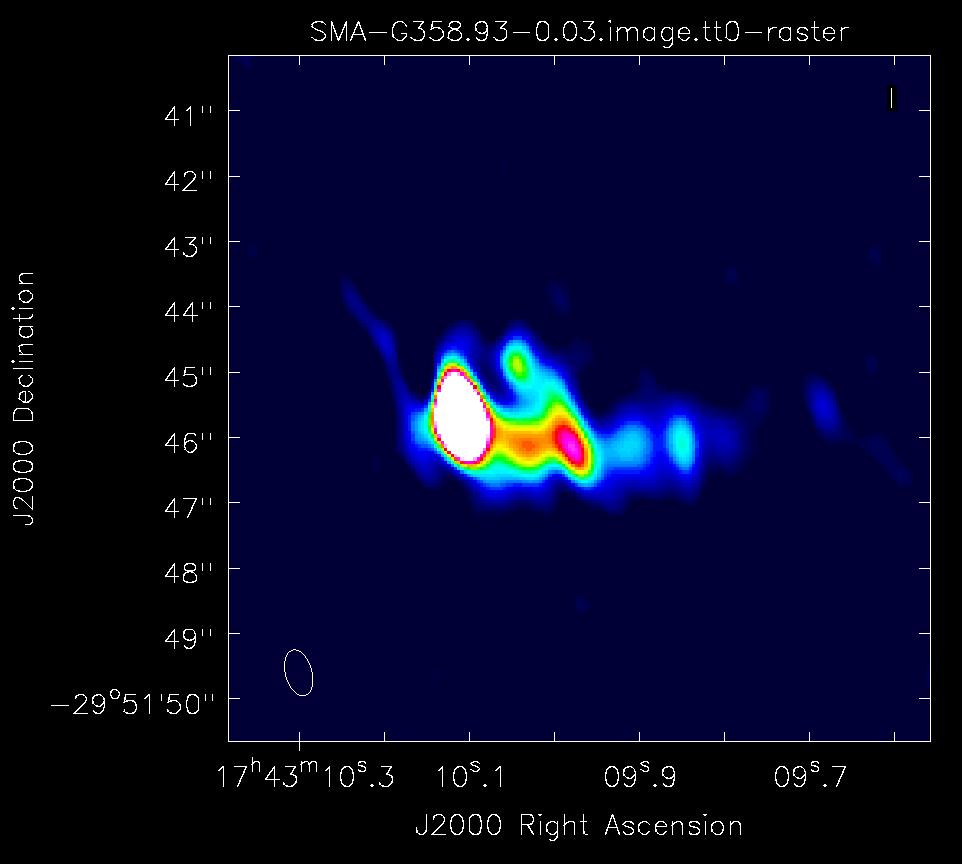
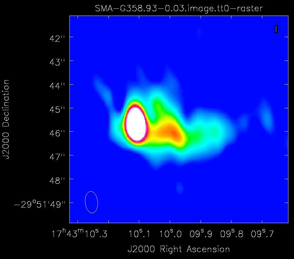 Fig. 20. SMA image of G358.93-0.03 at 210 GHz with Brigg's weight R=0 (left) and R=2 (right).
Left: The peak intensity and rms noise of R=0 weight image are 79.4 mJy/beam and 0.6 mJy/beam,
and FWHM beam is 0.72"x0.40" (15deg). Right: The peak intensity and rms noise of R=2
weight image are 89.7 mJy/beam and 0.45 mJy/beam, and FWHM beam is 0.91"x0.52" (5deg).
Fig. 20. SMA image of G358.93-0.03 at 210 GHz with Brigg's weight R=0 (left) and R=2 (right).
Left: The peak intensity and rms noise of R=0 weight image are 79.4 mJy/beam and 0.6 mJy/beam,
and FWHM beam is 0.72"x0.40" (15deg). Right: The peak intensity and rms noise of R=2
weight image are 89.7 mJy/beam and 0.45 mJy/beam, and FWHM beam is 0.91"x0.52" (5deg).
- Compare with ALMA 340 GHz image (Brogan et al 2019)
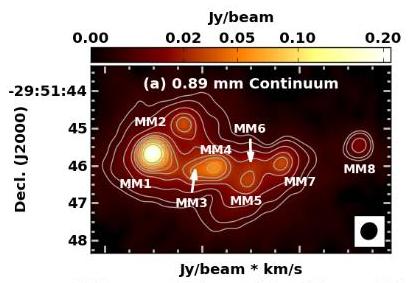
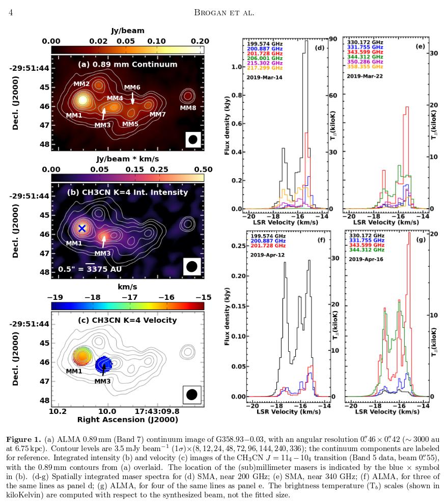 Fig. 21: ALMA 340 GHz (band 7) continuum image of G358.93-0.03 at an angular resolution
of 0.46" x 0.42", cut-pasted from original Fig. 1 (right) of Brogan et al. 2019.
Contours are 3.5 (?) mJy/beam (1σ) x ( 8, 12, 24, 48, 72, 96, 144, 240, 336); ....
The ALMA continuum components M1, M2, M3, M4, M6, M7, M8 appear to be detected with the SMA at
210 GHz; M5 and its surrounding extension appear to be not as strong as them in ALMA 340 GHz image.
rms of 3.5 (?) mJy/beam (1σ) for ALMA band 7 image appears to be
too high. Probably is a typo. According to SMA 210 GHz continuum image, this number more likely
0.35 mJy/beam. SMA's sensitivity of 0.45 mJy/beam at 210 GHz is close to ALMA band 7's sensitivity !?
Needs double check.
Fig. 21: ALMA 340 GHz (band 7) continuum image of G358.93-0.03 at an angular resolution
of 0.46" x 0.42", cut-pasted from original Fig. 1 (right) of Brogan et al. 2019.
Contours are 3.5 (?) mJy/beam (1σ) x ( 8, 12, 24, 48, 72, 96, 144, 240, 336); ....
The ALMA continuum components M1, M2, M3, M4, M6, M7, M8 appear to be detected with the SMA at
210 GHz; M5 and its surrounding extension appear to be not as strong as them in ALMA 340 GHz image.
rms of 3.5 (?) mJy/beam (1σ) for ALMA band 7 image appears to be
too high. Probably is a typo. According to SMA 210 GHz continuum image, this number more likely
0.35 mJy/beam. SMA's sensitivity of 0.45 mJy/beam at 210 GHz is close to ALMA band 7's sensitivity !?
Needs double check.
Step 13: Identify spectral lines and construction image cubes -
CASA tasks:
     clean (tclean)
     viewer
     ...
Usage of CASA-python-script module -
Image Callisto brightness distribution -
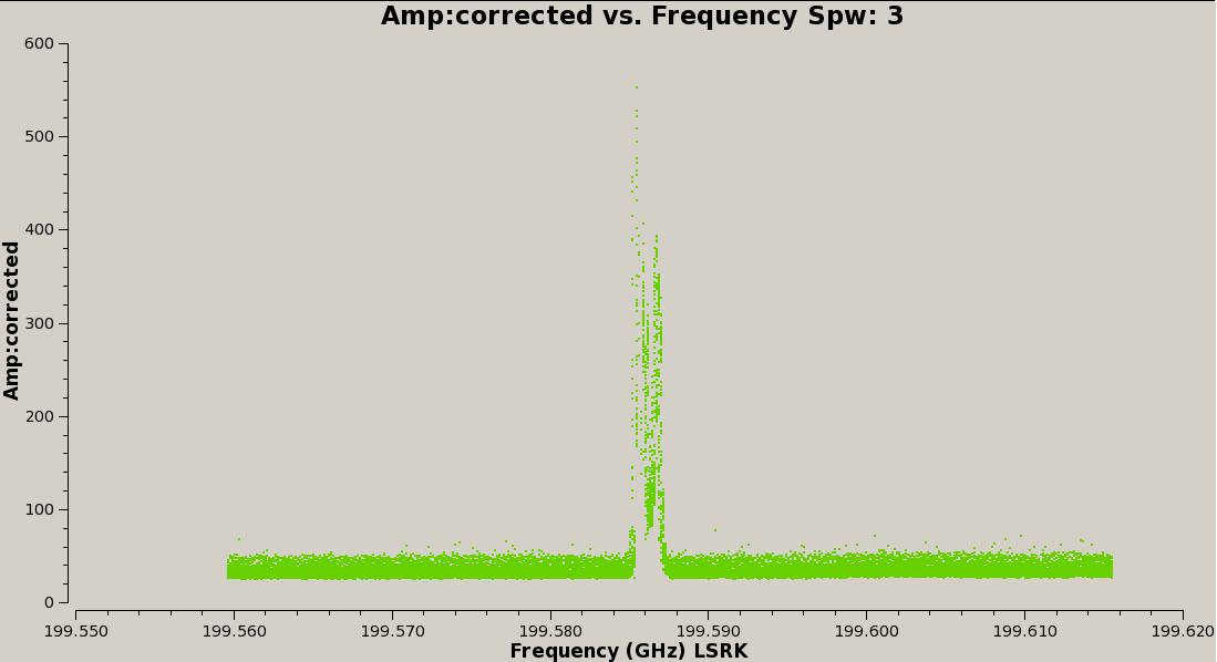
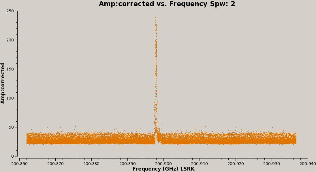

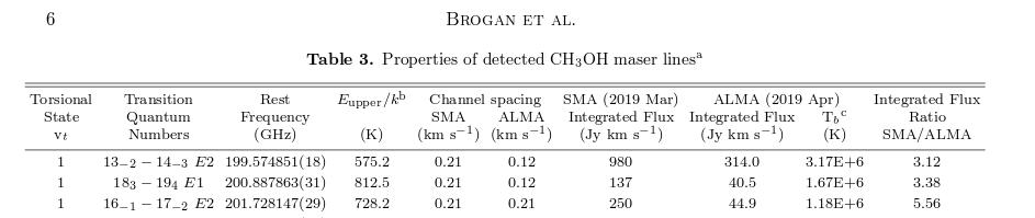 Fig. 22: CH3OH maser lines are identified for the three strong components near 200 GHz (top three panels)
which are listed in Table 3 of Brogan et al 2019 (Bottom). The spectra of these maser lines are also plotted in Fig. 1
of Brogan et al 2019 (see left of Fig. 21 above).
Step 14: Combine different array data -
Fig. 22: CH3OH maser lines are identified for the three strong components near 200 GHz (top three panels)
which are listed in Table 3 of Brogan et al 2019 (Bottom). The spectra of these maser lines are also plotted in Fig. 1
of Brogan et al 2019 (see left of Fig. 21 above).
Step 14: Combine different array data -
CASA tasks:
     ...
Usage of CASA-python-script module:
Skip this step for this example.
Step 15: Convert CASA images to FITS -
CASA tasks:
     ...
Usage of CASA-python-script module:
|
| |
| |
|

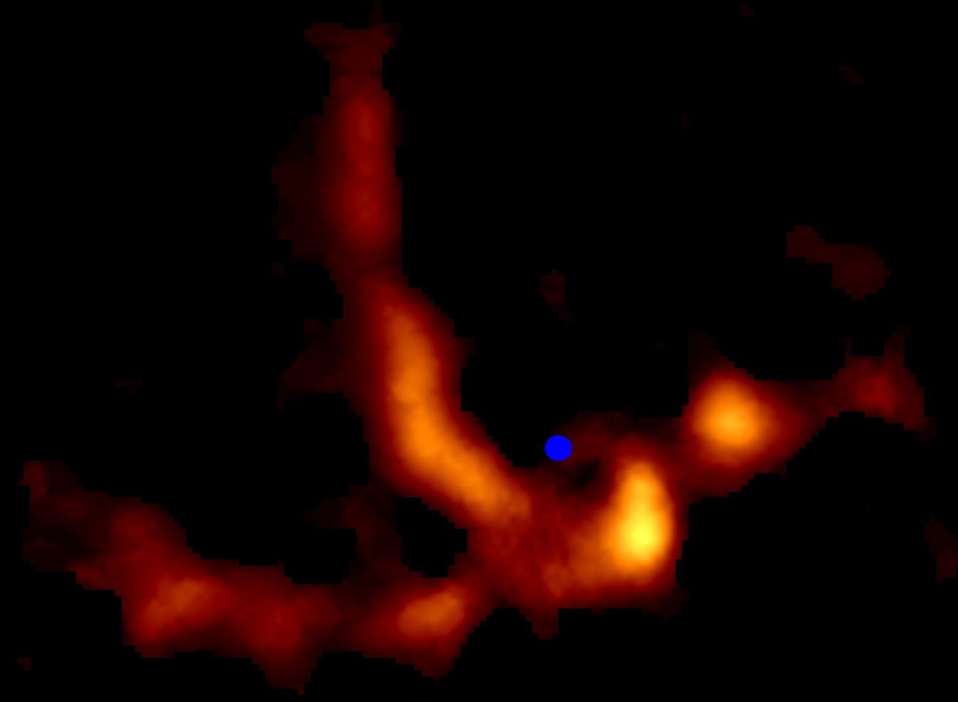
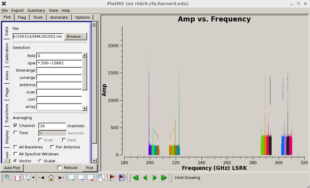 Fig. 0_1: the 16 spectra of field 0 (3c279) from SMA190314.ms.
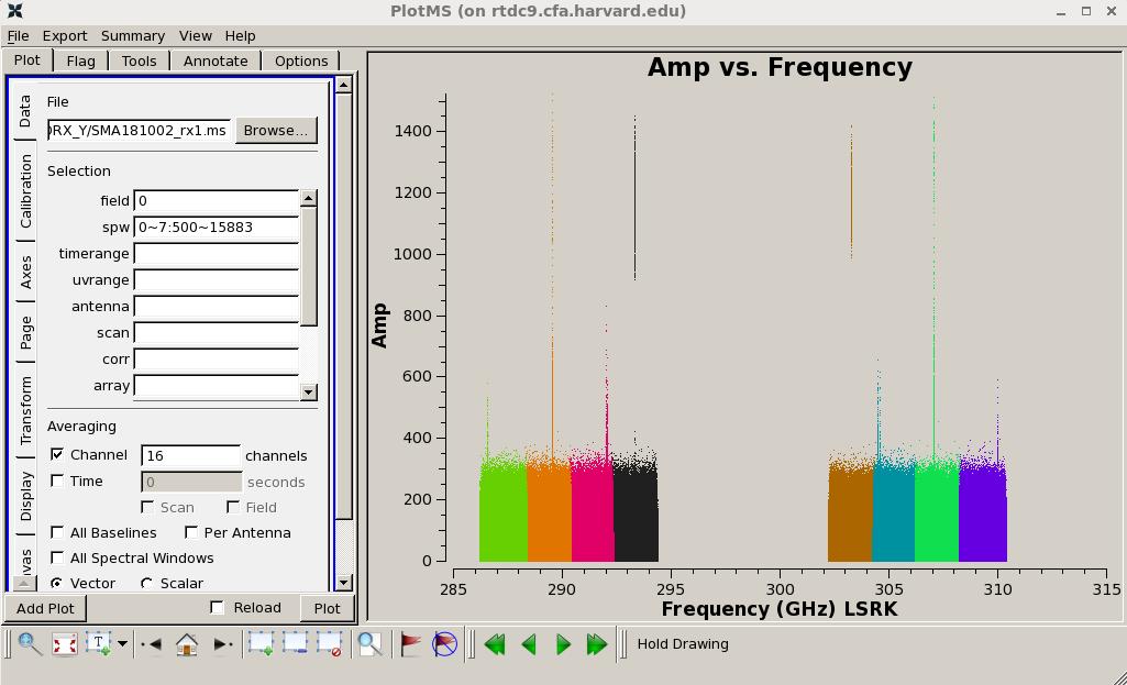 Fig. 0_2: the 8 spectra of field 0 (3c279) from SMA190314_rx1.ms.
 Fig. 0_3: the 8 spectra of field 0 (3c279) from SMA190314_rx2.ms.


